Sea level and ocean heat content
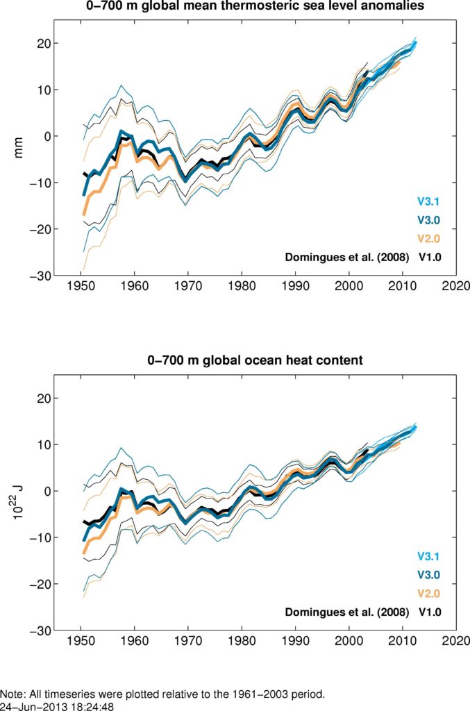
Global mean thermosteric sea level (GThSL) and global ocean heat content (GOHC) timeseries for the upper 700m
Download a print-quality pdf of this figure Download
If you have comments or queries about this, or would like to be added to the mailing list, send an email to catia.domingues@csiro.au
Version history: Global mean thermosteric sea level (GThSL) and global ocean heat content (GOHC) timeseries for the upper 700 m
(updates from Domingues et al., 2008)
| Recons. version | Period/Area available | Historical data | Argo data | XBT corrections | Climatology | Sat. altimeter EOF period / number of modes | Used in refs. |
|---|---|---|---|---|---|---|---|
| 3.1 | 1960-2012 65S-65N | EN3v1b 1960-2004 BO, CTD, XBT | CSIRO 2000-2012 | Wijfels et al. (2008), Table 1 | Wijfels et al. (2008) BO, CTD, Argo (monthly mean) | CSIRO 1993-2011 30 EOFs | |
| Click to download | Near-global yearly estimates smoothed by a 3-year running mean:
Note : As version 3.0 but with timeseries extending to 2012. Argo data downloaded on January 2013. |
||||||
| 3.0 | 1960-2012 65S-65N | EN3v1b 1950-2004 BO, CTD, XBT | CSIRO 2000-2011 | Wijfels et al. (2008), Table 1 | Wijfels et al. (2008) BO, CTD, Argo (monthly mean) | CSIRO 1993-2011 30 EOFs | (4), (5), (6), (7), IPCC AR5 (WGI Chaps : 3, 9, 10, 13) |
| Click to download | Near-global yearly estimates smoothed by a 3-year running mean:
Note : Bug fixed: missing square of one of the errors related to number of observations when combined in quadrature. Thanks to Didier Monselesan. |
||||||
| 2.0 | 1960-2009 65S-65N | EN3v1b 1950-2004 BO, CTD, XBT | CSIRO 2000-2009 (P. Barker) | Wijfels et al. (2008), Table 1 | Wijfels et al. (2008) BO, CTD, Argo (monthly mean) | CSIRO 1993-2006 30 EOFs | (2), (3), (8) |
| Click to download | Near-global yearly estimates smoothed by a 3-year running mean: | ||||||
| 1.0 | 1950-2003 65S-65N | EN3v1b 1950-2004 BO, CTD, XBT | CSIRO 2000-2009 (P. Barker) | Wijfels et al. (2008), Table 1 | Wijfels et al. (2008) BO, CTD, Argo (monthly mean) | CSIRO 1993-2006 30 EOFs | (1) |
| Click to download | Near-global yearly estimates smoothed by a 3-year running mean:
|
||||||
- Ocean temperature data
To estimate historical thermosteric sea level and ocean heat content (or potential temperature) for the upper 700 m, we use ocean temperature profiles available in the ENACT/ENSEMBLES version 3 (hereafter EN3; http://www.metoffice.gov.uk/hadobs/en3/) data set [Ingleby and Huddleston, 2007]. We discard profiles that have bad quality flags, have coarse vertical resolution, are shallower than the depth integration level or are from higher latitudes than 65°N and 65°S. We select only the temperature data that are clearly identified and measured by bottles (BO), conductivity-temperature-depth (CTD) profilers, and expendable bathythermographs (XBT) for which we can apply a correction for systematic fall-rate errors [Wijffels et al., 2008; Table 1]. We do not include temperature profiles from the remaining instrument types, of which a large fraction is from mechanical bathythermographs (MBT), because of their shallow depths and also lack of understanding of their systematic biases [Wijffels et al., 2008]. To complement the BOs, CTDs, and XBTs from the EN3 data set, we use the most recent version of our own quality-controlled Argo profiling floats (provided by P. Barker or J. Dunn), including data from floats corrected for pressure-sensor drifts [e.g., Barker et al., 2011; http://www.argo.ucsd.edu/Argo_data_and.html]. Given the increased availability of high-quality delayed-mode Argo data with time, we always update the entire Argo data set (from 2000 onwards) for our estimates. - Temperature climatology
We use a temperature climatology (provided by S. Wijffels) which mapping technique includes spatially-dependent terms and annual, semi-annual and linear trend terms at each grid point [Wijffels et al., 2008]. We believe this is superior to most other available climatologies in which all years are simply averaged together, yielding young median observation dates in the Southern Hemisphere and old median dates in the data-rich areas of the Northern Hemisphere. Attempts to resolve more than a linear trend in time were also considered, but estimates were poorly constrained by the data. - Thermosteric sea level and ocean heat content We convert temperature profiles into thermosteric sea level and ocean heat content relative to a number of fixed-depth reference levels, assuming climatological salinities from the World Ocean Atlas [Conkright et al., 2002]. We calculate anomalies relative to their monthly mean fields and map them into 1° latitude x 1° longitude grids for the ice-free ocean equatorward of 65°N and 65°S. Our deepest calculation is performed with respect to 700 m, because many XBTs measure to this depth [Wijffels et al., 2008]. To take advantage of the greater number of in situ observations in the upper ocean, the 0-700 m estimates are a sum of two depth integrations, 0-300 m and 300-700 m. Near-global timeseries are computed with equal-area weighting. Because of the sparse spatial in situ ocean coverage, particularly towards the earlier years of the record, the monthly reconstructed fields contain substantial noise which is then reduced by forming yearly averages smoothed by a three-year running mean filter.
- Reconstruction details In our reconstruction we use the sparse but relatively long record of thermosteric sea level anomalies to determine monthly amplitudes of leading empirical orthogonal functions (EOFs). The EOFs are used to model variability of the time-varying sea level and are calculated from satellite altimeter data (provided by CSIRO, here). An additional constant (essentially a spatially uniform field) is included in the reconstruction to represent changes in the global mean [e.g., Church et al., 2004; Church and White, 2006]. Before computing the EOFs, we apply an inverted barometer correction and remove annual and semi-annual signals as well as a global mean sea level trend from the altimeter data.
- Error estimates The reduced-space optimal interpolation formalism [Kaplan et al., 2000], designed to recover the large-scale robust patterns that can be derived from sparse data, provides estimates of errors on the basis of the data distribution and uncertainties in the in situ ocean observations (instrumental and geophysical errors) as well as ocean eddy variability determined from satellite altimeter data (provided by CSIRO, here). The latter two are combined in quadrature. The formal error estimates included in the downloadable files are for one standard deviation.
- XBT bias corrections We have significantly reduced systematic XBT fall-rate errors by applying the corrections proposed by Wijffels et al. [2008], listed in their Table 1. Further refinements in identifying and correcting XBT errors may be possible in the future. XBT bias corrections are a complex issue which is currently being addressed by an international working group (http://www.nodc.noaa.gov/OC5/XBT_BIAS/xbt_bias.html).
- Ocean heat content regression We convert the reconstructed near-global monthly gridded maps of thermosteric sea level into ocean heat content maps by using coefficients obtained from a spatially variable linear regression between observations of ocean heat content and thermosteric sea level. The regressions are calculated from the temperature profiles in 10° latitude x 10° longitude grid boxes (following the World Meteorological Organization squares). The resultant correlation coefficients are at least 0.99.
References
| (1) | Domingues, C.M. , J.A. Church, N.J. White, P.J. Gleckler, S.E. Wijffels, P.M. Barker and J.R. Dunn (2008), Improved estimates of upper-ocean warming and multi-decadal sea-level rise. Nature, 453, 1090-1094, doi:10.1038/nature07080. |
| (2) | Church, J.A., N.J. White, L.F. Konikow, C.M. Domingues, J.G. Cogley, E. Rignot, J.M. Gregory, M.R. van den Broeke, A.J. Monaghan, and I. Velicogna (2011), Revisiting the Earth’s sea level and energy budgets from 1961 to 2008, Geophysical Research Letters, 38, L18601, doi:10.1029/ 2011GL048794. |
| (3) | Gleckler, P. J., Santer, B.D., Domingues, C. M., Pierce, D.W., Barnett, T.P., Church, J.A., Taylor, K.E., AchutaRao, K.M., Boyer, T.P., Ishii, M., and Caldwell, P.M. (2012). Human-induced global ocean warming on multidecadal timescales. Nature Climate Change, 2, 524-529, doi:10.1038/nclimate1553. |
| (4) | Church, J. A., D. Monselesan, J. M. Gregory, and B. Marzeion (2013), Evaluating the ability of process based models to project sea-level change, Environmental Research Letters, 8(1). |
| (5) | Otto, A., F. E. L. Otto, O. Boucher, J. Church, G. Hegerl, P. M. Forster, N. P. Gillett, J. Gregory, G. C. Johnson, R. Knutti, N. Lewis, U. Lohmann, J. Marotzke, G. Myhre, D. Shindell, B. Stevens, and M. R. Allen. 2013. Energy budget constraints on climate response. Nature Geoscience, 6, 415-416, doi:10.1038/ngeo1836. |
| (6) | Hanna, E, Navarro, F., Pattyn, F., Domingues, C.M., Fettweis, X., Ivins, E.R., Nicholls, R.J., Ritz, C., Smith, B., Tulaczyk, S., Whitehouse, P.L., Zwally. H.J. Ice sheet mass balance and climate change: a state of the science review. Nature, 498, Pages: 51–59 DOI: doi:10.1038/nature12238. |
| (7) | Abraham, J.P., Baringer, M., Bindoff, N.L., Boyer, T., Cheng, L.J., Church, J.A., Conroy, J.L., Domingues, C.M., Fasullo, J.T., Gilson, J., Goni, G., Good, S.A., Gorman, J. M., Gouretski, V., Ishii, M., Johnson, G.C., Kizu, S., Lyman, J.M., Macdonald, A. M., Minkowycz, W.J., Moffitt, S.E., Palmer, M.D., Piola, A., Reseghetti, F., Trenberth, K.E., Velicogna, I., von Schuckmann, K., and Willis, J.K. Monitoring systems of global ocean heat content and the implications for climate change, a review, commissioned for Rev. of Geophysics (submitted 24/04/2013). |
| (8) | Griffies, S.M., J. Yin, S.C. Bates, E. Behrens, M. Bentsen, D. Bi, A. Biastoch, C. Boening, A. Bozec, C. Cassou, E. Chassignet, G. Danabasoglu, S. Danilov, C.M. Domingues, H. Drange, P.J. Durack, R. Farneti, P. Goddard, R. J. Greatbatch, J. Lug, E. Maisonnave, S.J. Marsland, K. Lorbacher, A. J. George Nurser, D.S. Melian, J. B. Paltero, B. L. Samuels, M. Scheinert, D. Sidorenko, L. Terray, A.M. Treguier, Y.H. Tseng, H. Tsujino, P. Uotila, S. Valcke, A. Voldoire, Q. Wang, S. Yeager, Xuebin Zhang. Global and regional sea level in a suite of interannual CORE-II hindcast simulations. To be submitted to Ocean Modelling. |
| (9) | Conkright, M. E. et al. World Ocean Atlas 2001: Objective Analyses, Data Statistics, and Figures, CD-ROM Documentation (National Oceanographic Data Center, Silver Spring, MD, 2002) |
| Ingleby, B., and M. Huddleston, 2007: Quality control of ocean temperature and salinity profiles—Historical and real-time data. J. Mar. Syst., 65, 158–175, doi:10.1016/j.jmarsys.2005.11.019. | |
| Kaplan, A., Kushnir, Y. & Cane, M. A. Reduced space optimal interpolation of historical marine sea level pressure. J. Clim. 13, 2987–3002 (2000) | |
| Wijffels, S.E., J. Willis, C.M. Domingues, P. Barker, N.J. White, A. Gronell, K. Ridgway, and J.A. Church (2008), Changing Expendable Bathythermograph Fall Rates and Their Impact on Estimates of Thermosteric Sea Level Rise. Journal of Climate, 21, 5657-5672, doi:10.1175/2008JCLI2290.1. | |
| Barker, P.M., J.R. Dunn, C.M. Domingues and S.E. Wijffels (2011), Pressure Sensor Drifts in Argo and Their Impacts. Journal of Atmospheric and Oceaninc Technology, 28, 1036-1049, doi:10.1175/2011JTECHO831.1 | |
| Church, J. A., White, N. J., Coleman, R., Lambeck, K. & Mitrovica, J. X. Estimates of the regional distribution of sea-level rise over the 1950 to 2000 period. J. Clim. 17, 2609–2625 (2004) | |
| Church, J. A. & White, N. J. A 20th century acceleration in global sea-level rise. Geophys. Res. Lett. 33 L01602 doi: 10.1029/2005GL024826 (2006) |