Sea level changes on a variety of space- and time-scales, and different measuring systems measure different subsets of the various components that make up the total picture. This is further complicated by the fact that different observing systems measure sea level in different reference frames (see table below), and that geological effects (long- and short-term) can move the reference frame and/or the sea level with respect to that reference frame! See our section “Why does sea level change” for more information on this.
The following table summarizes some of these issues:
Referenced to the centre of mass of the Earth (via a reference surface such as a reference ellipsoid). One effect of this is that, as the shape of the ocean basins is changing slowly with time, a correction needs to be made to the altimeter data for this.
Use of satellite radar altimeters to measure global sea surface height (SSH) has come a long way since the brief Seasat mission of 1978. Early missions measured SSH with an accuracy of tens of metres. More recent high quality satellite altimeter missions such as TOPEX/Poseidon (launched August 1992) and Jason-1 (launched December 2001) measure SSH to an accuracy of a few centimetres. These satellites were specifically designed to measure SSH to the highest possible accuracy.
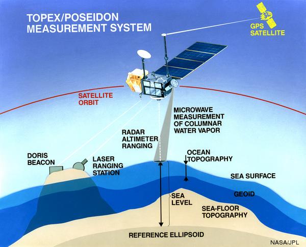
The essential parts of a satellite altimeter measuring system are:
A satellite in an orbit which repeats the same ground track very closely (within about 1 kilometre)
A radar system to measure the distance from the satellite to the sea surface to high accuracy. TOPEX/Poseidon and Jason-1 use two radar frequencies, Ku band (13.6GHz) and C band (5.3Ghz).
A tracking system capable of locating the satellite vertically at any time to within a few centimetres. Some of the components of such a system are:
Systems to locate the satellite, which are usually a combination of GPS, SLR (Satellite Laser Ranging), and the French DORIS system
A high quality gravity model
A model of the drag from solar wind and the atmosphere
Suitable software to combine all of the above
Other corrections to correct the range:
On the satellite:
A water vapour radiometer to measure the amount of water vapour between the satellite and the sea surface (the water vapour slows down the radar pulse, causing the raw measurement to be too long)
Measurement of the range at two frequencies to estimate the “ionospheric correction” – that is, the degree to which the radar pulse is slowed down by free electrons in the ionosphere
The troughs of waves contribute more to the radar reflection than the crests, so we need a correction for this. This is estimated from the wind speed and the wave height, both of which can be estimated from the characteristics of the returned radar pulse.
On the ground:
Ocean tide models to convert the raw altimeter measurement to the “detided” SSH
Estimates (from a model) of the atmospheric pressure. This is used to calculate a correction to the radar range to compensate for the fact that the atmosphere slows down the radar pulse
A correction is made for the “inverse barometer” effect, where sea level is depressed in areas of high atmospheric pressure, and vice versa
The picture below illustrates some of this.
Gravity/geoid models
The Earth is not spherical and both the gravity field and the (related) geoid (the equipotential surface) vary over the surface of the Earth. Oceanographic signals are small perturbations (typically less than a metre) on the geoid signal (which has a range of about 200 metres). Some early altimeter missions, such as the GEOSAT Geodetic Mission (see table below) were initially launched (by the US Navy) to measure the marine geoid, which then lead to estimates of the marine gravity field.
High precision satellite altimetry needs high quality gravity fields to estimate the perturbations in the satellite’s orbits caused by the spatial changes in the gravity field. This is at the stage now where the changes in mass (and hence gravity) caused by movement of the oceans by tides need to be included in the gravity models to get the best possible altimeter orbits.
Many Earth-observing satellites are in fairly low orbit (up to about 800 kilometres above the Earth’s surface), but TOPEX/Poseidon and Jason-1 used higher orbits (about 1340 kilometres) as this helped with orbit determination because the gravity field is a bit smoother at this higher altitude. Also there is less atmospheric drag on the satellite at this height. The payback for this is that the missions are more expensive because of the higher launch costs and the satellites have to work in a harsher radiation environment as there is less of the Earth’s atmosphere to protect them.
Satellite altimeter missions
Name
When
Orbit characterisitics
Comments
Skylab
1973
Experimental
Geos-3
1975-78
Mainly geodetic
Seasat
1978 (3 months)
800 km, 3-day repeat, inclination=78°, retrograde
Oceanographic
GEOSAT Geodetic Mission
1985-1986 (18 months)
800 km, non-repeating
Geodetic
GEOSAT ERM (Exact Repeat Mission)
1986-1990
800 km, 17-day repeat, inclination=78°, retrograde (included Seasat orbit)
Oceanographic
ERS-1 other phases
various, 1991 on
Various modes, including a brief geodetic phase
ERS-1 phases C & G
1992-1993 and 1995-1996
800 km, 35-day repeat, inclination=81°, retrograde, sun-synchronous
Oceanographic
TOPEX/Poseidon
1992-2005
1,340 km, 10-day repeat, inclination=66°, prograde
First truly high quality oceanographic altimeter
ERS-2
1995-2003
As for ERS-1 phases C&G
GFO (GEOSAT Follow On)
2000-2008
As for GEOSAT
Follow-on of GEOSAT ERM
Jason-1
2001-present
As for TOPEX/Poseidon
Follow-on of TOPEX/Poseidon mission
Envisat
2002-present
As for ERS-2
Jason-2
June 2008 – present
As for Jason-1
Follow-on of TOPEX/Poseidon and Jason-1
Notes on the table:
Heights are heights above the Earth’s surface
“Inclination” is the angle between the plane of the satellite’s orbit and the equator. A satellite going over the poles would have an inclination of 90°
A satellite in a prograde orbit (e.g. TOPEX/Poseidon) is always moving east relative to the Earth. A satellite in a retrograde orbit (e.g. GFO) is always moving west relative to the Earth
A sun-synchronous orbit (ERS-1/2, Envisat) is one in which the satellite passes over any location on the Earth at the same local time every cycle.
The repeat time (or cycle length) is the time between subsequent overpasses of the same point on the Earth’s surface.
TOPEX/Poseidon was moved into a new orbit (same inclination and cycle length, but moved longitudinally) in August 2002.
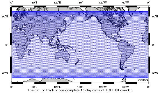
TOPEX/Poseidon
Plot of the TOPEX/Poseidon ground track
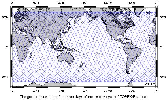
Plot of the first three days of TOPEX/Poseidon ground track
It may be easier to see what is happening from this subset (the first three days) of the the 10-day cycle.
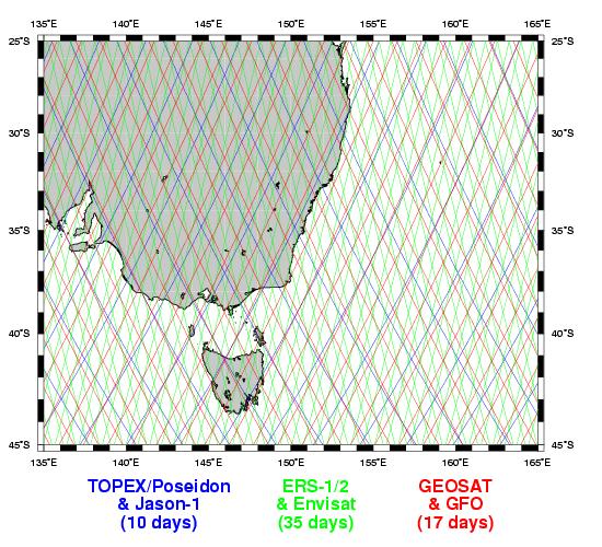
Plot of all ground tracks in the SE Australian region
This plot shows the tracks of three different satellites over the south-eastern part of Australia.
Some facts about the TOPEX/Poseidon (and Jason-1) orbit
Each 10-day (actually 9.916 days) cycle consists of 127 revolutions (“orbits”), which can be broken up into 127 ascending and 127 descending half-orbits (“passes”). For a prograde orbit like TOPEX/Poseidon, ascending passes go South-West to North-East, and descending passes go North-West to South-East.
Each complete orbit (full revolution) takes approximately 1 hour and 52 minutes.
Orbit height is about 1,340 kilometres – it varies slightly because of the shape of the Earth (a slightly pear-shaped, flattened sphere) and the (small) eccentricity of the orbit. For comparison, the radius of the Earth is about 6,370 kilometres.
The inclination of 66.04° means that the maximum latitude it reaches is 66.04°(N or S). Note that the ground track spans Drake Passage (between the southern tip of South America and Antarctica), one of the major choke points in the oceanic circulation. This was one of the design criteria for this satellite.
The ground track repeats within ±1 kilometre of the nominal track.
The orbit was chosen to maximise the potential for solving for the most important ocean tides. Major advances in estimation of tides and understanding of the underlying science have come from this mission.
Altimeter orbits are usually chosen with as low an eccentricity (i.e. as near-circular) as possible – but it is usually non-zero as this parameter is what is used to “lock” the orbit into an exactly repeating pattern. The TOPEX/Poseidon orbit had an eccentricity of 0.000095.
Please note that we have upgraded our processing of the earlier missions (TOPEX/Poseidon and Jason-1) to what is known as ‘GDR-D’ standard.
The most important difference is that orbits for all missions are now in ITRF2008 (Altamimi et al, 2008). Orbits for TOPEX/Poseidon and Jason-1 are the GSFC std1204 orbits (Lemoine et al, 2010). The ITRF2008 orbits that are supplied with the data are used for OSTM/Jason-2.
Other significant differences are that all missions now use the GOT4.8 tide model. The Chambers et al (2003) SSB correction is used for TOPEX/Poseidon. The Tran et al (2010) SSB correction is used for Jason-1.
These changes make a noticeable difference to the shape (but not the overall trend) of the GMSL curves. They make little difference to regional patterns.
Tide Gauges
The measurement of long-term changes in sea level from tide gauges involves the following for any one site:
Joining together data from a number of different instruments, which may include:
Highs and lows and their times measured by eye off a tide staff and written by hand in a book
A modern state-of-the-art acoustic tide gauge recording automatically every six minutes
Several generations of technology in between
Referencing them all to the same vertical datum, taking into account movements around the wharf area where they are installed and any movements of the structures that they were mounted on
Referencing the site’s vertical datum to some standard vertical datum
Fortunately for us most of this work has been done at the Permanent Service for Mean Sea Level (PSMSL). The University of Hawaii also maintains an archive of tide gauge data. For our work we normally use the monthly average data as we are mainly interested in the long-term behaviour, but higher frequency data is needed for some applications. Some high frequency data is available from the PSMSL and UHSLC, but much of it is in national archives, such as Australia’s National Tidal Centre (NTC). A combined data product of high frequency tide gauge data is available through the Global Extreme Sea Level Analysis (GESLA) project.
Tide gauge-derived SSH records are subject to contamination by vertical movement, which can take various forms:
Long-term and more-or-less constant, such as changes caused by Glacial Isostatic Adjustment (rebound from the last Ice Age)
Short term, e.g. the Boxing Day (2004) Tsunami, which was caused by an earthquake
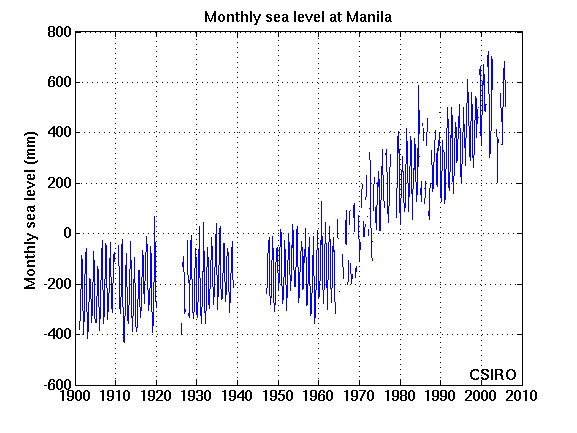
Varying in time over periods of years or decades. This can be caused by sinking of piers because of unstable foundations or sinkage of land through, for example, groundwater pumping. A good example of the latter is the tide gauge record for Manila in the Philippines:
Tide gauge record at Manila
In recent years a lot of effort has been going into installing GPS receivers at, or very close to, high quality tide gauges to try to estimate this vertical movement directly and then correct for it. Some of the GPS records are now able to provide useful estimates of this. See for example GLOSS and TIGA.
Paleo Indicators
Our estimates of sea level before the earliest tide gauge records (17th century) are dependent on what are referred to as “paleo” indicators. These are indicators (usually natural, but sometimes man-made) whose age, and whose height, relative to modern-day sea level can be measured accurately enough to give worthwhile measurements of past sea level. While these measurements are not nearly as accurate as modern instrumental techniques they can still give useful restraints on sea level histories due to the long time period.
Some of the natural markers are:
raised beaches and wave cut notches
fossil shells and vegetable matter
submerged salt marshes
Some of the man-made markers are:
Ancient Roman (~1st century AD) fish tanks (“Piscina”)