Document Version: 16 July 2020

1
Overview

The
Open Pit Simulator (OPS), also known as SIROMODEL, was originally developed for
the Large Open Pit Mine Slope Stability Project and has subsequently undergone
many enhancements.

This application allows the user to create a
structural model of a section of an open pit excavation. It also includes a
multi-function discrete fracture network (DFN) generator. This allows
deterministic discontinuities such as bedding planes and faults and daylighting
or confirmed joints (called deterministic joints) to be added to this model.
Random joints (called stochastic joints) can be generated upon each simulation
based on the statistical parameters for each joint set. Termination settings
can be used to control the way various discontinuity sets terminate against
each other. The software will determine the intersections of all these
structures and the presence of all complete blocks within the model, known as a
block model. Statistics on each block
can be calculated and the blocks can be viewed individually or as an ensemble. Rigid block limit equilibrium
stability analyses can also be performed. For confidence in interpreting
results from simulations using stochastic joints, a batch of simulations can be
run constituting a Monte Carlo
analysis. The aforementioned analysis tools can then be used on this batch of
simulations.

The block finding algorithm used in Siromodel
has been designed for handling finite persistence structures. It therefore does
not utilise optimisations or efficiencies available to other algorithms that
are limited to handling infinite persistent structures. If the structures you are
modelling consist almost entirely of persistent structures, then Siromodel may
not be the optimal solution and one of the variety of spreadsheet or
application based codes currently available may be more suitable.

1.1      About This Version

Feedback and bug reports should be sent to OPSFeedback@csiro.au . 

For a full list of changes, visit http://www.csiro.au/3dvision/Siromodel/ReleaseNotes.txt

Each instantiation of OPS will check for
updates.

1.2      Installation

Down load a full
installation or upgrade patch from https://research.csiro.au/msci/projects/mining/siromodel/
and run it on your machine. Your existing license key will work with this
updated version. To request additional license keys, please email OPSFeedback@csiro.au. The first start-up of the application may
take some time as necessary files are extracted, but subsequent start-ups
should be significantly faster.

 

1.3
Quick Start

Start OPS.

Select File ‘ New Model.

Create a multi-bench model by entering the
desired parameters (example shown in Figure 1).

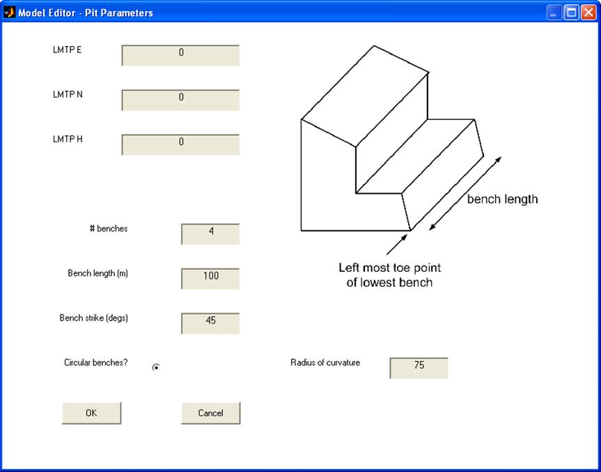
Figure 1 Pit parameters for the ‘Quick Start’ example.

Enter bench parameters for each of the benches as desired. See Figure 2 for an example.

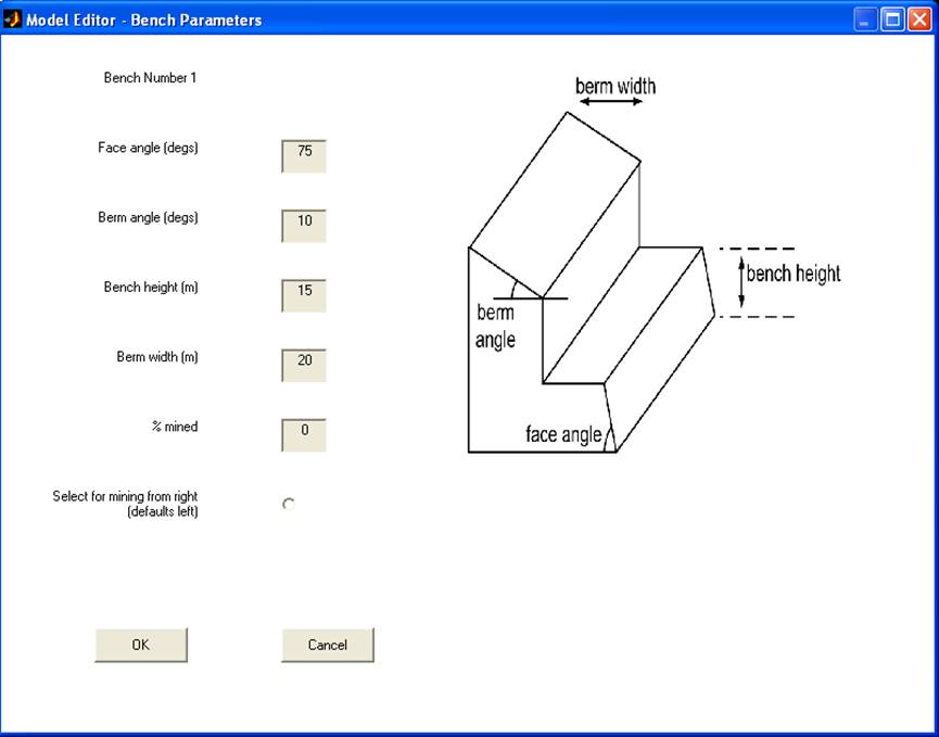
Figure 2 Bench parameters for the ‘QuickStart’ example.

Note that for creating models with many benches, it may be more desirable
to define the model parameters ‘off-line’ by directly editing an OPS model
parameter text file. See Figure 14 and section 3.1.1 for more details. To create a model parameter file for your current
model, select File
‘ Save ‘ Model ‘ Save OPS parameter file. You can
examine the contents and formatting of this file with any text editor

Define Beds or Faults by using the Edit menu. For example, select Edit ‘ Beds, and then select Edit Polygons, Edit Properties and
then Bench-face
geometry. Hold the mouse over each edit box to receive a tool-tip (see Figure 3 for an example of bed parameters).

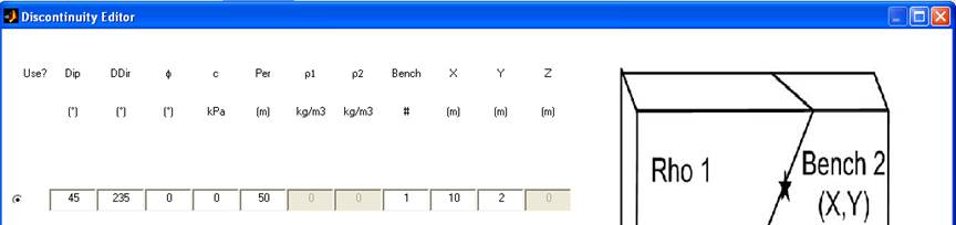
Figure 3 Example of bed parameters

Import deterministic joints using File ‘ Load ‘ Joints‘ Deterministic Joint Polygons.
These could be in the form of a Sirovision Discontinuity file.

You can import joint set statistical parameters
using File
‘ Load ‘ Joints‘ Stochastic Joint Statistics. These could be in
the form of a Sirovision Discontinuity Set Statistics file. Alternatively,
define sets of joints to be stochastically generated by selecting Edit ‘ Joints ‘ Edit Stochastic Joint Stats. See Figure 4 for an example of some joint set parameters.

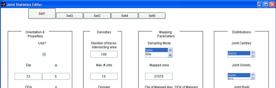
Figure 4 Example of joint parameters

Use Options
‘ Stochastic Joint Conditioning to
control the way the stochastic joints are generated with respect to the
imported deterministic joints.

Now select Tools ‘ Run Simulation, and
leave the number of projects set to 1. Finally, select the destination for the
project file. An Analysis Window and Block Visualiser window will eventually be
generated.

You can now perform some analysis of this
‘block model’ by selecting Tools ‘ Block Model Analysis. Experiment with the Options menus to see what capabilities are present. Refer to section 3.3 for
more details.

For worked examples, see section 5 towards
the end of this manual.

 

1.4
Getting
Started

1.4.1
Workflow

The workflow can be summarised as follows:

 

 

1.4.2
Performance

The time required to generate a block model is a function of the
complexity of the simulation being conducted, which is a function of several
parameters. These include the complexity of the pit geometry being used (e.g.
user-defined pit geometry versus an imported triangulation), the complexity of
the discontinuities being inserted (e.g. planar representation of a bed versus
a triangulated surface representation), and the number and interactivity (i.e.
density of discontinuity intersections) of the discontinuities being used. As a
guide, the example project that accompanies this software (BFJExample.opp)
involves a user-defined pit with 5 benches, 100 discontinuities resulting in
400 blocks and now takes approximately 1 minute to run on a Pentium D 3.2GHz
machine with 1GB RAM.

1.4.3
Terminology
& Concepts

The following terms
are commonly used throughout this document:

 

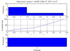
As stated above, the
first task is to create a model of the section of pit being analysed. For all
model types except the closed surface, the bounding volume consists of sides, a
back and a base (see Figure 5). These sides designate bound surfaces, in that any blocks in
contact with these surfaces are not free to slide. Other surfaces are
considered to be free surfaces.

 

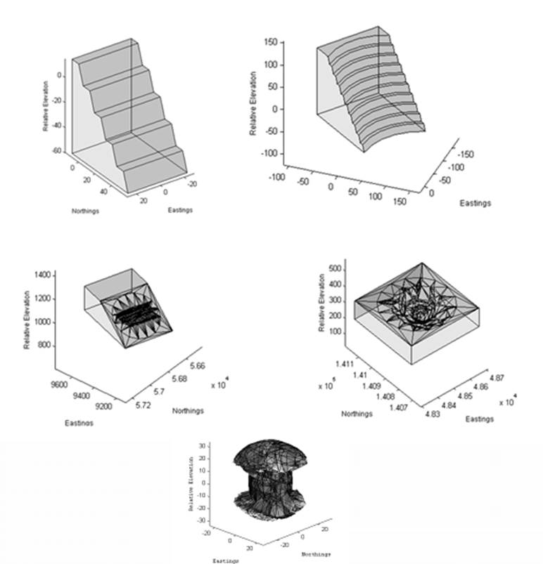
Figure 5 The Bounding
Volumes for various geometries (linear at top-left, circular at top-right,
surface – pit section at middle left, surface ‘ pit shell at middle right,
closed surface at bottom). For each type except the closed surface, the sides
& base are bound surfaces (i.e. rock blocks in contact with these surfaces
are deemed immovable). For the closed surface case, all surfaces are considered
free.

The introduction of
geological information such as discontinuities, domains, water table etc is the
next step to perform. Note that the following options are available:

‘       Introduction of beds and faults as either

o
planes
specified by orientation and trace point position

o
surface
triangulations created by third party software

‘       Introduction of joint sets as either

o
polygons
created by third party software

o
stochastically
generated joint sets (generated at the start of each simulation) by specifying
the joint set parameters

‘       Introduction of water table as either

o
plane
specified by orientation and trace point position

o
surface
triangulation created by third party software

o
pore
pressure (spatially gridded) data

‘       Introduction of geological domains as a surface
triangulation created by third party software

Once some or all of
this detail is in the model, the user can tailor the options for the
simulation/s being performed. This includes setting intersection terminations
for discontinuity sets, setting limits on the maximum and minimum sizes of
structures to include in the simulation, and specifying the so-called ‘active
depth’, or the depth below the surface to deem structures as active.

Once the simulations
are complete, a block model analysis can take place including all of the block
models that have been generated.

2
Theory

This software utilises a polyhedral modelling
algorithm which is based on the boundary definition of polygons. Such
algorithms for use in the geo-technical domain have been discussed recently in
Jing (2000), Lu (2002) and Elmouttie & Poropat (2010). Consult these
references for details however, in essence, the algorithm computes the
vertices, edges and therefore the faces resulting from the intersections of all
finite persistence polygons defined in the
model. With this information, the polyhedra (rock blocks) that form from the
faces can be computed. These polyhedra are not limited in complexity in terms
of number of faces or shape (see Figure 6).

The polygons represent
joints, fractures, beds, faults and other discontinuities that are present in
the rock mass. A realisation of these structures is referred to as a discrete
fracture network (DFN). The software accommodates importation of DFN generated
from third party software but also contains its own DFN generator (see
discussion on Stochastic Joint Statistics
for details). The accuracy of the models used in the software is clearly a
function of how well the generated DFN’s represent the real structure in the
rock mass.  

Stability analysis is
performed using a Limit Equilibrium (LE) method (Hoek & Bray 1981) combined
with the Goodman & Shi (1985) classification scheme
(Type I  or Unstable, Type II  or Stable with friction and Type III  or Stable
without friction). The full
geometry as defined by the block model is considered via a modified Warburton
vector analysis (Warburton 1981) in determining whether a block is removable.
The surface properties are then considered (friction angle, cohesion and pore
pressure) to determine how to classify the block. Note that only the
Mohr-Coulomb shear strength model is supported at this stage.

Pore pressures are
calculated if a water table (phreatic surface) has been imported or defined.
The depth below the water table to the centroid of a block is used to determine
the pressures at the surfaces of that block. Modification to these pressures is
possible via the importation of geotechnical domains. For each domain, a pore
pressure ‘coefficient’ can be assigned which can attenuate the pore pressure in
that domain from 0 to 100%. Alternatively, rather than specifying of a water
table, a gridded set of pore pressure values can be imported. Either way, the
pressures are used in the LE analysis to determine the upthrust force acting on
the sliding surfaces and the pore pressure forces acting on the non-sliding
surfaces.

Blocks can be bolted
in place, the assumption being that the means are available to overcome the
reported ‘removal force‘ acting in the direction of the reported ‘removal
vector‘ (see 3.2.3). It is assumed that the depth of the bolt is
sufficient to prevent all blocks that may be obstructed by the bolted block
from failing.

 Static forces (e.g. for simulation of a
seismic event) specified as either a force in a given direction or as one
acting along the individual sliding vector of the blocks are also considered in
the LE analysis. Blocks are assessed individually so no account is taken for
‘group failures’. However, the ability to perform iterative or progressive
failure analysis exists and so the algorithm can ‘peel’ away multiple layers of
removable blocks until only stable blocks remain.

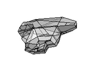
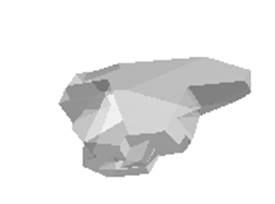
Figure 6 An example of a
complex block detected by the algorithm (with and without edges shown)

To establish some degree of confidence that
the essential characteristics of the ‘blocky’ rock mass are being captured, the
use of multiple ‘realisations’ of joint structures (and hence multiple
realisations of blocks) is highly recommended. The number of such ‘simulations’
needed will depend on the confidence one has in the input data (e.g. the need
for running separate simulations with different properties for hidden, major
through-going structures such as faults), the variations seen in the field for
the physical characteristics of the structures (e.g. variance in dips, friction
angles etc), the geometrical characteristics of the structures being modelled
(e.g. joint density, interactivity etc) and the type of analysis being
performed (e.g. in-situ block size estimation, LE analysis etc).

As a general rule of thumb, one should use
a sufficient number of simulations to properly ‘fill’ the probability mass
function or histogram for the parameter being investigated (Vose
2001). To illustrate this point, Figure 7 shows
the number of blocks found for multiple simulations of the BFJExample.opp
project (provided with this software). Clearly, using 10 simulations has failed
to identify an obvious shape to the distribution, but using 200 simulations
shows a more convincing result.

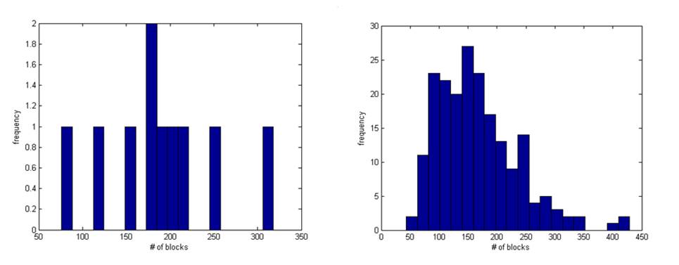
Figure 7 Histograms
representing block numbers for 10 simulations (left) and 200 simulations. The
latter clearly shows a more complete (i.e. less coarse) histogram yielding more
confidence in estimation of the expected value and likely variance.

 

3
Functionality

3.1      The
Control Window

 

The Control window consists of a set of
menu controls and a display area (see Figure
8). The window is used to visualise the pit
model and any bedding, fault or deterministic joint discontinuities that have
been defined. It also allows you to control the main functionality of the
software. However, other windows can be generated depending on the type of
analysis you perform.

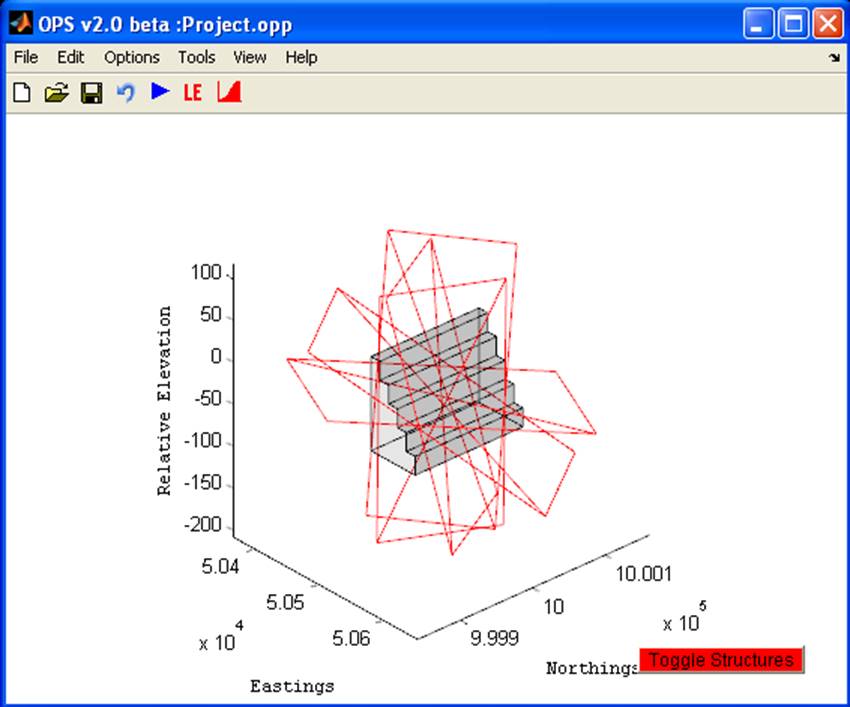
Figure 8 The OPS Control
window.

The menu system
will now be discussed in detail.

3.1.1
File Menu

The
File menu controls allow you to create, load & save data.

New Project ‘ start a new project.

New Model OP ‘ create a new user defined
open pit model whilst retaining any pre-existing discontinuities. The user
defined model types are ‘linear’ or ‘circular’ (see Figure 5). Such a model requires the user to specify
all relevant geometrical information such as number of benches, bench
dimensions etc. Strike is defined using the left most portion of the model, not
the average strike (important to note for curved models). A user defined model
can be edited at any time to alter the dimensions of the pit. This is not the case
for other model types (i.e. imported surface models). Note support for such
surface models is limited to quasi-linear pit sections (curvature of the
surface is not too great) or full pit shells. This is because OPS tries to
‘stitch’ the surface to a bounding box, using a sloped side for a pit section
or the top of the box for a pit shell. A bounding box around the model geometry
is used for the stochastic structure generation. Therefore, to avoid boundary
effects such as biases, one should define a bounding box large enough to
account for this (see Edit ‘
Bounding Box). A
good rule of thumb is to increase the dimensions of the model in each direction
by the maximum structure size of interest.

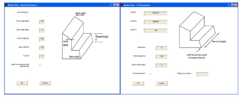
Figure 9 The interfaces for editing the pit (left) and bench (right)
parameters of a model

New Model UG ‘ (for UG module only) create
a rectangular prism bounding volume to house an imported void or user defined
void. For this type of model, all six faces of the prism are defined as bound
surfaces and only blocks daylighting against the void will assessed
kinematically (or those adjacent to these for progressive failure analysis).
You can also use this menu item to convert a model previously defined using the
open pit model editor into an underground model (however, if multiple benches
are present, only the geometry of the first bench will be used).

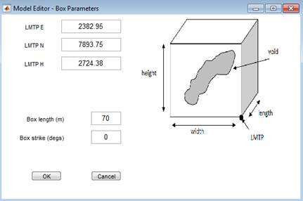
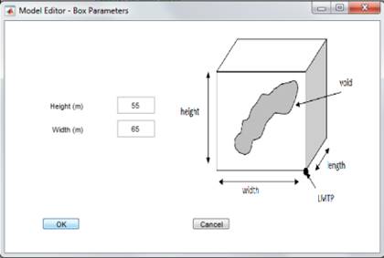
Figure
10 The interfaces for editing the parameters of an underground model

 

Load ‘ loading or importing of all data
is performed in this menu

Model ‘ load a Sirovision 3D file, DXF surface triangulation, OPS model
parameter file or SlopeModel xml file to use as a pit model geometry.

 

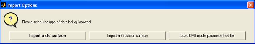
Figure 11 The dialog box for choosing the type of model to import

Selecting
one of the first two options will create a non-editable ‘surface’ type model.
Although the importing of full pit shells is now supported, normal practice is
to use a section of a pit (usually consisting of several benches) for the pit
model. Surface models can not be edited as they are
based on predefined surface information. Surface models can be either pit
sections, pit shells or closed surfaces, all assumed to be triangulated
surfaces. For the closed surfaces, the software will check that the selected
data is a closed manifold surface (i.e. every edge of the triangulation is
shared by exactly two facets). For closed surfaces built such that base facets
are horizontal and side facets are vertical, then these will be defined as
boundary surfaces. For arbitrary shaped closed surfaces, the entire surface is
treated as a free surface requiring a stability analysis (i.e. there are no
bound surfaces).

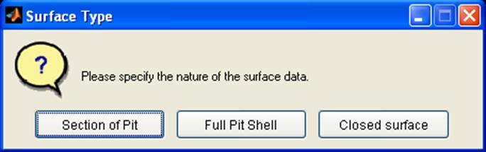
Figure 12 The dialog box for specifying the geometry represented by the
surface data.

 

Note that
the use of surface triangulations to define the pit geometry imposes a large
time penalty on block model simulations. This is because compared to a
user-defined geometry the number of polygons in such a model is significantly
larger. To alleviate this problem, the software will request the number of
points to retain. Keeping this as low as possible will improve computation
times.

Further, in the case of Sirovision data,
the option of creating an idealised user-editable model (type ‘linear‘ or ‘circular‘) based on the surface data will be presented (Use
a best fit circular model). This should be
selected whenever possible as it greatly simplifies the pit geometry and
therefore can help to reduce computation times. Note that the user will almost
certainly need to ‘tweak’ the model parameters for this ‘best fit’ model. To
assist in this regard, one can overlay the actual Sirovision surface data on
the model using File ‘
Load ‘
Toggle Overlay Surface.

 

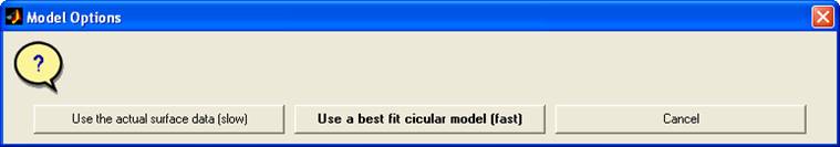
Figure 13 The dialog box for simplifying the raw data to a user-editable
circular bench model.

Alternatively, one can also load an OPS
model parameter file. This is a formatted text file containing the model
parameters for a user-defined model of type ‘linear’ or ‘circular’. An example
is shown in Figure 14.

 

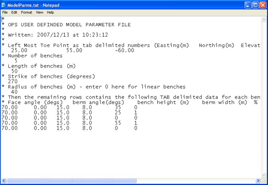
Figure 14 The contents of a
typical OPS model parameter file.

A summary of the model creation work-flow
discussed above is presented in Figure 15.

Figure 15 Model creation
work-flow summary

Project ‘ load an OPS project file (*.opp).

Joints ‘
load stochastic joint statistics or deterministic (realised) polygons

Load Stochastic Joint Statistics ‘ load
a joint statistics file created with OPS or a Sirovision Discontinuity Set
Statistics file. OPS joint statistic files are text files where each row of
text describes statistical properties (e.g. mean and standard deviation of dip
and dip direction) for a set of joints to be stochastically generated in OPS.
See section 3.1.2 for a description of these fields. Sirovision Discontinuity Set
Statistics files are text files created using the File-Export-Discontinuity Set
Statistics feature (in Sirovision 3.4.1)

Load Deterministic Joint Polygons – load a joint polygon file. This gives the
user the ability to enter a realisation of joints generated by third party software.
The option to ‘grow’ or extrapolate these discontinuities so that they are
fully or partially persistent throughout the model geometry is also provided.
File types supported are Sirovision Discontinuity text file, JointStats ASCII,
DIPS ASCII and DXF (polygon) files. Some comments on selected formats follow.

Sirovision
Discontinuity text file

The format required for the Sirovision
Discontinuity text file is an 8 column tab delimited format with columns
containing the following data for each joint:

Dip (degs), Dip
Direction (degs) Joint ID (numeric) Joint Set ID
(numeric) Trace Length or maximum chord length (m) Centroids Easting (m)
Northing (m)  Elevation (m)

JOINTSATS
file

The text based (non-XML) format is supported.

DIPS

The format for the DIPS text file is assumed to
be oriented in terms of Dip and Dip Direction. This should be indicated in the
file via the phrase DIP/DIPDIRECTION appearing on a separate line somewhere in
the header information. Only orientation data is used and it is assumed the
first 3 data columns are:

ID (numeric) Dip (degs)  Dip Direction (degs)

It is assumed no spatial data is available and joints
are generated with the imported orientations using a random process throughout
the simulation volume. If spatial data is also available, then it is
recommended you reformat the DIPS file as a Sirovision Discontinuity text file
(MS Excel can be used for this). Even if Trace Length data is not available,
dummy values can be inserted into the text file. OPS will then allow you to
choose specific persistence options during the importation process.

DXF file

It is assumed that the individual joints are
defined as separate polygons in this file (i.e. please avoid importing
triangulated polygons).

 

Surface discontinuity ‘ load a surface
triangulation representing a bed, fault or void in the form of a Sirovision 3D
image or DXF (triangulation) file. Multiple or bifurcating surface geometries
should be separated and imported individually as separate dxf files. Also,
please be aware that the importation of any surfaces which possess facets that
are coplanar with bounding volume facets can cause the erratic behaviour in the
block finding algorithm. Voids are assumed to be closed surfaces. If you use an
unclosed surface, just be aware that the block modelling algorithm may not
correctly keep the void ’empty’ of all blocks. For the case of bed or fault
importation, single surfaces should be loaded individually. Note that because
of the inevitable asperities in such surfaces, the limit equilibrium stability
analysis performed on any blocks sliding on these surfaces will most likely
deem the blocks to be geometrically stable. Therefore, for both computational
efficiency and algorithm robustness, it is advised that the simplest possible
representation of a surface be used and if possible, one without asperities.
One option for simplifying surface is to specify a lower number of points to
retain in the triangulation. Another option for simple (quasi-planar) surfaces
is planar representation. Either define the plane in OPS using the Edit
menu items or
use the option provided during import to represent your imported surfaces as
planar polygons.

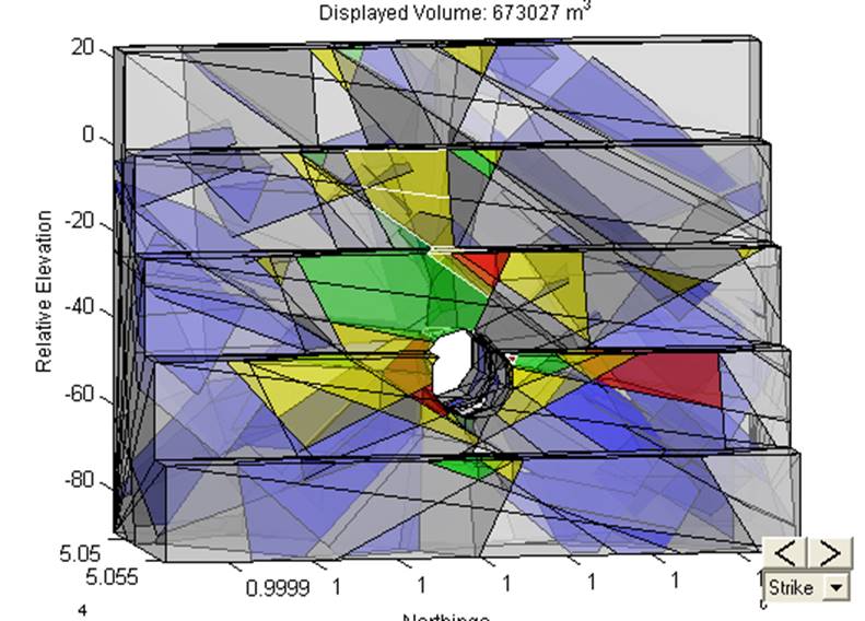
Figure 16 An example of a block model incorporating a void.

Domain ‘ load a DXF file of a closed triangulated surface representing a geotechnical domain. Using the simplest
(lowest resolution) possible representation will ensure computational
efficiency. For each domain, a density and pore pressure coefficient can be
specified. The latter can serve as a method of attenuating the pore pressures
introduced to the model via File ‘
Load‘
Water (e.g. to simulate a ‘perched’ water table, ensure the pore pressure
coefficients for domains below the water affected region are set to zero). See
section 3.2.1 to learn how to create domains
within OPS using the Block Visualiser window.

The
option to also import a Domain Shape surface is provided. This is a
triangulated surface for the representative shape of the domain (e.g. a neutral
surface). If provided, this surface will be used by the DFN generator to
generate joint orientations in folded sets (see the discussion of folded sets
in Edit ‘
Joints for more details).

Water ‘
options for introducing water to the model.

Water Table – either load a DXF surface
triangulation file or define a plane representing a water table. This option
will delete any previous water table or pore pressure data in the model. If a
water table is specified, then the pore pressure at each block will be
calculated as the total pressure associated with the height of the water table
above the centroid of the block and the atmospheric pressure.

Pore pressures ‘ import a text file containing
pore pressures specified for certain spatial locations in 4 column
tab’delimited format. Spatial data needs to be specified as Eastings, Northings
and elevations in metres. Pressure data should ideally be in Pascals although a
dialog box is presented to allow conversion of other units. Importing pore
pressures will delete any previous water table or pore pressure data in the
model. If this option is chosen, the pore pressure at each block centroid will
be determined using the input pressure data and spatial interpolation (as of
version 4.8.8). The pore pressure grid displayed in the main figure is only
indicative and, particularly for large grids, only a random sample of data is
shown.

Toggle Overlay Surface ‘ see section 4 Common functions.

OPS parameter files ‘ load OPS
discontinuity parameter data

Bed Parameters ‘ load an OPS bed
parameter file. Bed and fault parameter files are text files where each row of
text describes properties (e.g. dip, dip direction, friction angle etc) of a
discontinuity to be deterministically generated in OPS (see
3.1.2 for more details).

Fault Parameters ‘ load an OPS fault
parameter file.

Save ‘ saving or exporting of all data
is performed in this menu

Project ‘ save the current work in an
OPS project file. The file format has been optimised since OPS V2.0 and so
older versions of OPS are unable to load these projects.

Model ‘
save the pit geometry model

Export model as DXF ‘
export the pit model geometry as an Autocad Release 14 DXF file. Both polygon or triangle based
representations are now supported.

Save OPS parameter file ‘ save the model parameters as an OPS parameter text file.  For surface models, only the parameters
associated with the ‘frame’ used to support the triangulation are saved.

Export Blocks ‘ export the polyhedra in
various formats, including polygonal faces, triangulates faces and as component
tetrahedra. Both DXF and text file export is supported. Some more details are
as follows:

DXF export ‘ export the polygonal or
triangulated face blocks as an Autocad Release 14 DXF
file (assumes a full simulation has been performed ‘ see
3.1.4 for more details on simulation mode options). Each block is assigned
as a separate DXF ‘block’ entity. Block faces can be represented at polygons or
triangles.

Text file export – writes out two text
files containing data on the polygonal/triangulated or tetrahedral
representations of the blocks in the project. One file contains a list of
vertices of the blocks, the other contains a list of indices (referring to the
vertex file) corresponding to each face/facet on the block. A block identifier
is also provided to allow association of each tetrahedra with the original
blocks.

Export Discontinuities ‘ export the bed, fault and joint data as an Autocad Release 14 DXF, DIPS format, JointStats XML or
generic format (e.g. as used by 3DEC). The latter consists of tab delimited columns of Easting, Northing,
Elevation, dip, dip direction and radius. Either
original polygons or those truncated against the bounding volume can be
specified.

Beds ‘ export bed planes and surfaces

Faults
‘ export fault planes and surfaces

Joints
‘ export deterministic and stochastic joints

All Discontinuities
‘ export all of the above

Export Voids ‘
export the triangulated void data as an Autocad Release 14 DXF. If multiple voids are present, user will be prompted as
to which ones to export.

OPS parameter files ‘ save OPS
discontinuity parameter data

Bed Parameters ‘ save a text file containing the current bedding parameters.

Fault Parameters ‘ save a text file containing the current fault parameters.

Joint Statistics – save a text file containing the current joint set parameters.

Intersection Segments ‘ save a text file
containing information for all intersection segments in the current model. An
intersection segment is defined by a pair of vertices representing the
intersection of any two polygons in the model. For each segment, the
intersecting polygons are identified as well as orientation information for the
segment itself.

Export Traces ‘ export drill cores (Figure
17),
scan line, rectangular or circular
windows (Figure 18) or
an exposure based trace map of the current model as a UDEC, 4-column ASCII or
DXF file. This assumes that at least a partial simulation involving
discontinuity generation has been undertaken (see
3.1.4). Statistics on the trace properties are reported as an ensemble (Figure 19) or
on a set basis if the ‘Trace Set Parameters’ control is activated (Figure 20).
These facilities can be used to assess the correspondence between the simulated
joint structures and those observed in the field. Note that the
histogram/stereonet shows joint (not trace) orientations. A fracture intensity
map (referred to as a P21 statistic) can also be generated (Figure
21). The
units for this are fracture length per unit area of exposure (or m/m²).
To change the colour range used in this image, right-click on the colorbar.

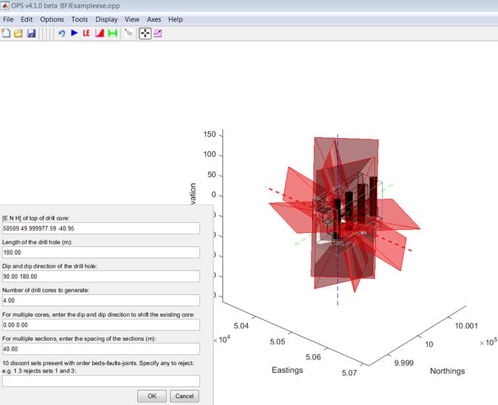
Figure 17 Use the move and
scale tool to interactively define drill cores, alternatively type in the
parameter in the input boxes.

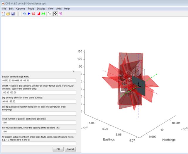
Figure 18 Use the move and
scale tool to interactively define rectangular or circular cross sections, alternatively
type in the parameter in the input boxes.

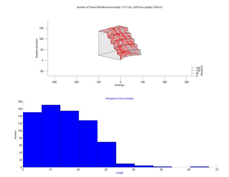
Figure 19 An exposure trace
map and trace length histogram

 

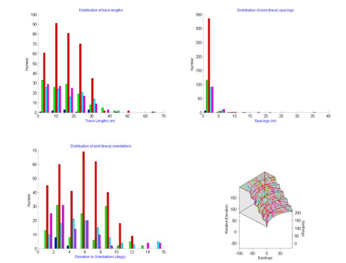
Figure 20 Trace set
parameters

 

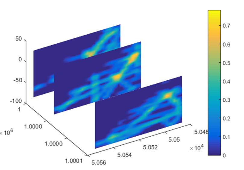
Figure 21 Fracture intensity maps
generated for 3 sections

 

 

Block Statistics ‘ create a text file containing block statistics.
Header comment lines begin with the asterisk sign (*), data for each block is contained
in a row which is tab delimited column format. The columns that are written out
are:

Block identifier number

Number of faces

Number of vertices

Non-release flag (1 for blocks that are
attached to non-release surfaces, 0 for others)

Block Centroid Easting (m)

Block Centroid Northing (m)

Block Centroid Elevation (m)

Block Surface Area (m²)

Block Volume (m³)

Removal Vector Easting (m)

Removal Vector Northing (m)

Removal Vector Elevation (m)

Removal Vector Dip (degs)

Removal Vector Dip Direction (degs)

Factor of safety

Exposed face area (m²)

Topple Flag (0 for safe, 1 for topple)

Number of fractures within this block

Total Fracture Area (m²)

Note
that the fields shown in red are only calculated for removable blocks. The
value NaN (not-a-number) is substituted here for
non-removable blocks.

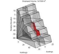
Monitor Points ‘ allows the user to save
a set of monitor (or hstory) points used in numerical
modelling packages. Currently limited to generating points on bench faces.
Support for DXF, text file and SlopeModel xml is provided. 

Figure 22 Example of monitor points generated on the bench faces for export.

 

Save plot data ‘ see section 4 Common functions.

Project Properties ‘ present a summary
of the current project, including the Options used. Note that an asterix (*) next to the number of blocks present indicates
several iterations of the algorithm were needed to derive a block model. A
double asterix (**) indicates that the maximum number
of iterations was reached and the block model may not be reliable.

 

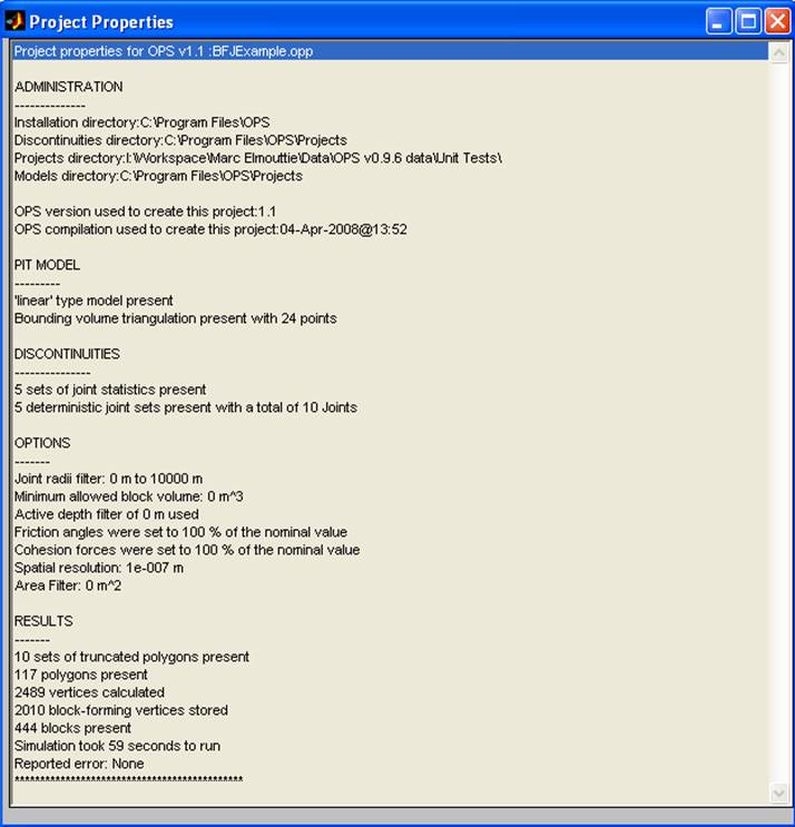
Figure 23 The ‘Project Properties’ window summarises the important
characteristics of the current project.

Batch ‘ various options for batch
processing of projects

Rerun full simulations for multiple projects ‘ allows the user to select multiple OPS projects and rerun the
simulations using the current Options settings. For example, one may wish to change the joint shape
representation (Options ‘
Joint representation) and rerun all the
previously run simulation to determine the significance of this parameter.
Another example might involve changing the size or area filter parameters prior
to rerunning the simulations (Options ‘
Filters). Note that altering options listed
below the line in the Options menu does not require full simulations to be re-run. Rather, the
user should select File ‘
Load‘
Batch ‘
Rerun LE for multiple projects in this case.

Rerun full simulations for multiple projects with different pit geometry ‘ as above but also allows the user to specify a different pit
geometry. For example, one may have created a number of simulations using a
certain user defined bench geometry, and then wish to see the effect of
altering that geometry (say, by mining a particular bench or benches). To do
this, one should define a model parameter file (see Figure 14) for
the altered geometry prior to selecting this function.

Rerun LE analyses ‘ as above except only the
limit equilibrium analyses will be re-run. This may be useful if one wishes to
tweak the LE related options (those listed below the line in the Options
menu of the control window) and re-run
previously calculated LE analyses. Also available is the ability to rerun the
LE analysis for the current project multiple times and applying randomly
generated deviations to friction angle and cohesion of surfaces (see Options
‘
Set standard deviation for phi and cohesion).

Export DFN from multiple projects ‘ allows
the discontinuities from a batch of projects to be written in various formats ‘
see #ExportDiscontinuities.
Rotations about the principal axes can be
specified in degrees and are applied as clockwise rotations when viewed from
the respective positive axis.

Export Properties from multiple projects ‘ this
will call the previously mentioned Block Statistics function in batch
mode.

Export Block Geometries/Properties from multiple projects ‘ this
will call the previously mentioned Export Blocks and Block Statistics
functions in batch mode.

Block Model Analysis ‘ this will allow you to
load multiple OPS project files or a single *.opa
file (OPS Block Model Analysis file) to perform some statistical analyses based
on multiple realisations. A separate ‘Block Model Analysis’ window will be
generated (see 3.3). By default, no blocks are filtered from the analysis at the start
of a block model analysis. The user must use the Edit menu within the Block
Model Analysis window to restrict the analysis to specific block types.

 

 

 

 

3.1.2    Edit Menu

The Edit
menu is used to modify the current model.

Bounding Box ‘ edit the dimensions of the bounding box used by the DFN generator. This
can be useful to ensure the space near the surfaces of interest (e.g. bench
faces) is populated with equal probability by discontinuities on both sides.   

Model ‘ edit the parameters (e.g. bench
dimensions, number of dimensions etc) for a user defined (linear or circular) model.
No editing facilities are provided for surface models (i.e. models created with
Sirovision data or DXF files). Note that editing model parameters (unlike
editing discontinuity parameters) will automatically delete the results from
any previous simulations from memory. Cancelling out of the model editor at any
stage will avoid this deletion.

Beds ‘ Edit the properties of individual
bed polygons or surfaces. Only friction angle and cohesion can be edited for
surfaces. For user defined polygons, two types of geometry are accommodated. A
‘world coordinates’ geometry is the standard Easting, Northing & Elevation
coordinate system. If the model is a user defined one (linear or circular),
then a ‘bench geometry’ is also supported whereby the user can specify the
bench number, distance along the toe of the bench and distance above the toe
for which a coordinate measurement has been taken (see Figure 24). Only one type of geometry can be used for
either beds or faults in a given project.

 

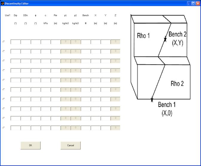
Figure 24 The Bed editor as
it appears when using ‘bench geometry’ coordinates

If these parameters are saved to file
(using Save ‘
OPS parameters ‘
Beds), the file format (no longer a tab
delimited) contains the parameters shown in Figure 25. Please note that file formats for OPS data
(such as Beds, Fault and Joint parameters) are subject to change and are only
provided to allow importing/exporting/editing of data for a current OPS
version. No backwards compatibility for importation of these files is guaranteed.

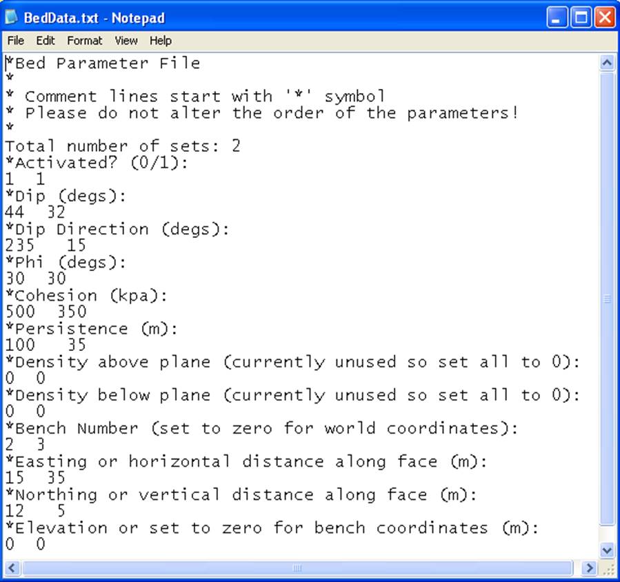
Figure 25 The file format
used for the bed and fault parameters.

The user can also delete selected beds by using
the ‘Clear Polygons’ option.

Faults ‘ Edit the properties of
individual faults. This is similar to Edit ‘
Beds.

Stochastic Joint
Stats ‘ Edit the statistical parameters used
by OPS to create a set of joints. It is assumed that the values used have been
corrected for the various biases such as orientation, truncation and censoring
biases (e.g. Zhang & Einstein 1998). The size bias is automatically
accommodated in the statistics used which are a function of the choice of
sampling mode. This assumes the space around the
surfaces of interest (e.g. bench faces) are populated by discontinuities on
both sides with equal probability. This can be ensured by adjusting the
bounding box used by the DFN generator (see Edit ‘
Bounding Box).  Currently, only areal, line and
volume (i.e. full) sampling are supported. Loading an older project will
automatically populate these parameters with default values. Of course, the
user needs to check these parameters for adequacy.

The joint
set generator currently only supports the Baecher Model (Baecher & Einstein 1977) and slight variants thereof.
This model assumes circular joints are distributed uniformly throughout the
simulation volume with their total number adhering to a Poisson process (i.e. a
binomial distribution tailored for large numbers of low probability events).
The joints are modelled as discs with log-normally distributed radii (Figure 26). The traditional assumption in the
literature has been that the choice of radial distribution function should
match that of the observed trace length distribution, hence the editor allows
specification of the former. However one should note that strictly speaking,
the radial distribution should not be assumed to be the same as the trace
distribution and it is only through analytical or numerical integration of the
specified trace distribution function that a true predictor of radial
distributions can be derived (Tonon & Chen 2007).
This facility is currently unavailable in OPS.

The joint
set generator utilises expressions relating the expected moments of the radial
distribution to their trace length counterparts for the assumed radial
distribution (Chan & Goodman 1983; Lyman 2003) assuming areal or line
sampling methods are used (Warburton 1980). These expressions place constraints
on the relationship between the mean (E(L)) and standard deviation (s(L)) of the trace lengths (s(L) > κE(L) with κ = 0.28 for areal and 0.20 for line
sampling). If the constraint is violated (e.g. the user specifies a standard
deviation which is too small to be consistent with the expressions), the
standard deviation of the trace lengths will be adjusted. Note that OPS v1.2
and prior utilised areal sampling calculations from Chan & Goodman (1983).
These expressions were found to contain an error which over-predicted the radii
so one may notice a marked reduction in the sizes of the joints generated in
this current version of the software. In any case, it is advised that the user
should inspect the generated trace lengths associated with the intersections of
the joints with a surface (e.g. using File ‘
Save‘
Export Cross-Section) to ensure the model replicates the field adequately.

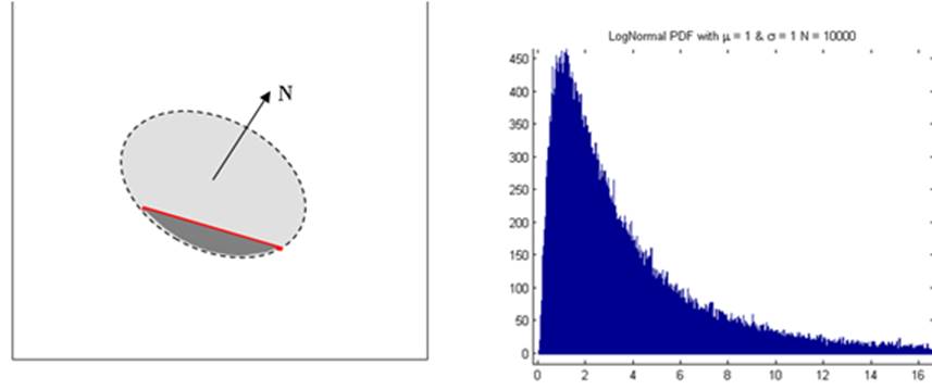
Figure 26 At left, an
idealised joint intersecting a plane (outcrop). The normal vector is shown and
the ‘exposed’ portion of the disc is darkened with the trace shown in red.  At right, a typical lognormal distribution.

Joint sets can terminate against each other
(Figure 27)
according to the user defined settings (use Options ‘
Enforce Termination Precedence). To reduce
computation time, the software represents the joints as low order polygons and
currently allows the user to select either triangles, rectangles or hexagons
(use Options ‘
Joint Representation). The hexagonal representation incurs a penalty of approximately 400%
computation time compared to the triangular representation.

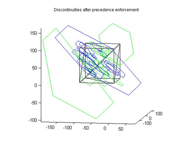
Figure 27 Two sets of
hexagonal joints with the first set (blue) having termination precedence over
the second (green).

 

The joint
statistics editor is shown in Figure 30.
Please use the tab buttons at the top of the editor to access the data for
different joint sets. The fields in the editor will now be discussed.

The Length/Diameter field refers to the mean value for the traces measured in the
field, or for volume sampling the mean diameter of the joints. The Δ field refers to the standard deviation of this
parameter.

The
Orthogonal Trace Spacing/True Spacing field now refers to
the mean bias corrected spacing measured orthogonal to the mean trace
orientation or for volume sampling, the true spacing measured in the joint
set’s normal direction. A facility to correct line sampling spacings (normally
measured along the sampling line itself rather than orthogonal to the trace)
has been provided. Note that if the Orthogonal Trace Spacing
field is set to zero, the software will randomly distribute the discontinuities
throughout the specified domain (note that a domain of 0 represents the entire
pit model). If the spacing is non-zero, the software will generate spacing
bands utilising a model specified in the Joint Spacings
field. The Δ field must also be provided although it is
unused in the exponential spacing model.

The Zone Parameter allows the user to control the width of the zones centred at each
of the spacing bands. The use of the parameter is dependent upon the type of
distribution specified in the Zone Dist field. For the uniform distribution,
the Zone
Parameter is used as the distance on either side of the band which
is populated uniformly. For the normal distribution, the Zone Parameter is used
as a standard deviation of normally distributed joints centred at each band.
Setting the Zone Parameter to zero
will force the DFN generator to use a single joint per spacing band (i.e.
over-riding the value in Max # Joints).
This can be useful when replicating geometries used by other software packages
which assume persistent joints.

The f and c fields refer to the friction angle (degs) and cohesion (kPa) of the joints respectively.

The Number of Traces/Joint density field
requires the observed number of traces for either the area that was mapped or
the scan line that was used. For volume sampling (see below) this field
requires a joint density to be entered. This parameter will control the number
of joints generated within the specified volume. If a domain has been assigned
to this set, then joint generation will limited to the domain volume. If no
domain assignment is made, the bounding box surrounding the model geometry is
used. The user must ensure that, particularly for the latter case, boundary
effects (e.g. biases) are accounted for (see Edit
‘
Bounding Box). 

The number of joints per set is calculated
by the software in different ways, depending on the sampling mode used. For
line and areal sampling, the number is calculated using stereological
principles and based on the number of traces mapped. For volume sampling, the
joint density (number of joint centroids per unit volume) is explicitly
specified by the user and the number of joints is calculated based on the
volume of the model. If the user also specifies the imported domain to use for
a particular set, then the number of joints is calculated based on the volume
of the domain. 

The Max #Joints field
allows the user to optionally specify a maximum number of polygons to be
generated for each joint set, thus limiting the computation time (Figure 28). If the Max #Joints field is set to zero,
the software will determine the predicted number of joints based on the
observed number of traces entered and the joint set geometry, in accord with
the Poisson distribution function. This, however, will result in a large number of
joints and therefore increase computation time and system requirements
considerably. Further, the enforcement of this limit is only performed
at the end of the fracture generation process to minimise the influence on the
statistical parameters of the set. Therefore, please be aware that joint set
generation can be slow if the implied fracture frequency is high, even with a
small Max
#Joints value. For example, if one is modelling a rock mass with
volume around 1000000 cubic metres and sets the Joint density
parameter (for volume sampling) to 1 m-3 and the Max #Joints value to 1000, then the joint set generator
will still perform all calculations on 1 million generated joints but only
return 1000 of these for the analysis. 

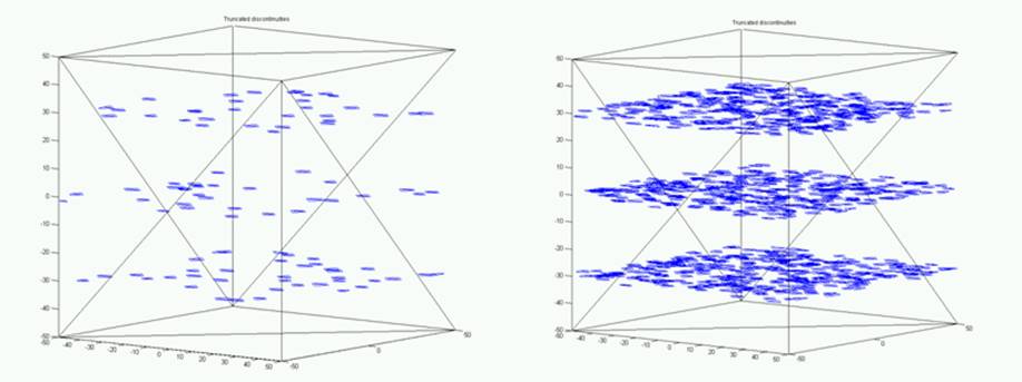
Figure 28 The effect of
increasing Max #Joints
parameter from 100 to 1000 in a spaced joint model (banded).

The Domain identifier can be used to
force generation of a joint set to a particular domain (see Figure 29) which has been imported via File ‘
Load ‘
Domain. Note that as in the field, the
intersection of joints against a boundary will impose censoring biases. To
completely avoid such effects, one should define domains well within a bounding
volume (e.g. cube) and limit the joint generation to this domain. In other
words, the bounding volume should be large enough to account for these boundary
effects (see File ‘
New Model). Any sampling of this DFN (e.g. via File
‘
Save ‘
Export Traces) will not be subject to censoring bias.

The Termination Prob. Against Domain field allows
you to enforce termination of the joint set against the domain boundaries.
Specify 1 for termination of 100% of joints, 0 for no termination.

The Folded Set?
option button allows you to specify if this set should be generated with
orientations following the local pole orientations of a surface representing
the shape of the domain. Choosing this option has implications for compatible
joint spacings models ‘ see the discussion on Joint Spacings for details. It assumes
a domain for the set has been specified using the aforementioned Domain
identifier. If this radio button is selected, the orientations specified in the
Dip
and DDir fields will be interpreted
as relative to the local pole direction of the domain’s shape surface (see Figure 29). If no domain shape surface was supplied during importation of the
domain geometry (see File ‘
Load ‘
Domain) one will
be calculated using the average of the upper and lower domain surfaces, each
being estimated via a projection method. If this is not adequate for your
domain geometry, a domain shape surface should be provided during importation
of the domain geometry.

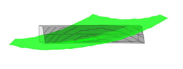
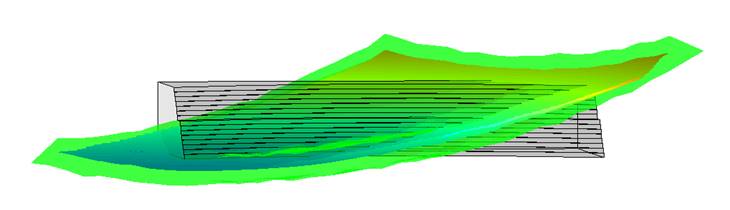
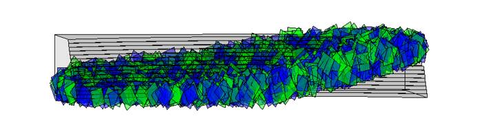
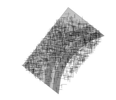
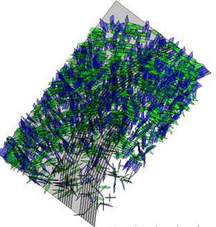
Figure 29 Joint set generation
within a domain. (a) shows the domain boundary and (b) including the shape
surface. (c) a realisation of two sets confined to the domain. (d) the case of
mutually orthogonal sets with orientations referenced to world coordinates,  (e) mutually orthogonal sets for the case
when folded sets are requested – the orientations are now referenced to the
local pole geometry of the domain.

 

The Sampling Mode field allows the user to
choose between areal sampling, line sampling and volume sampling options. The
former two refer to the traditional techniques used to map joint traces on
outcrops. The latter refers to an idealised case where one has 3-dimensional
information and is therefore aware of the joint density within a rock mass
(i.e. no inference based on outcrop mapping is required). For scan-line
sampling, please ensure the specified scan-line dip and dip direction are
consistent with the specified ‘mapped area’ dip and dip direction (that is,
scan-line coplanar with the area). If using the scan-line mode to represent
borehole or tunnel data, please refer to Mauldon
& Mauldon (1997) regarding additional corrections
for orientation bias associated with these forms of mapping. 

The Joint Centres field currently only
allows a Poisson distribution to be used.

The Joint Orients field currently only
allows a normal distribution to be used.

The Joint Radii
field supports lognormal, exponential normal and uniform distributions. For
exponential, the Std length field is ignored as
only the mean is required. For normal and uniform distributions, the user is
prompted to enter the joint size parameters directly as inversion of trace
parameter data is not available for these distributions.

The Joint Spacings
field allows the user to choose between banded, normal, exponential and uniform
distributions to generate the spacing bands. All spacings are measured relative
to the mean joint set normal direction. Therefore, the behaviour of the
following spacings models may not be consistent with folded sets, particularly
if the domain geometry is severely folded.

The banded
spacing model forces the joints to reside within regularly spaced bands
separated by the stated spacing value. The positions of the bands are varied
randomly for each simulation using a uniform distribution varying between 0 and
half the stated spacing value and the band spacings are varied using a normal
distribution with standard deviation specified in the Standard Deviation in Spacing value. For larger standard
deviations, the banded model will approach the normal distribution model.

The normal
distribution model requires both the Spacing
and Standard Deviation in Spacing data to generate the spacing bands.

The
exponential distribution model requires only the Spacing data to generate the spacing bands.

The uniform
distribution model requires a minimum and maximum spacing to be specified.

Note that
the joint generator will continue to ‘populate’ the available spacing bands
until the total number of joints exceeds either the predicted number (according
to a Poisson process) or the user specified maximum (Max #Joints field).

The Zone
Distribution field allows the user to choose between ‘uniform’ and ‘normal’
distribution types. See the discussion on the Zone Parameter for details.

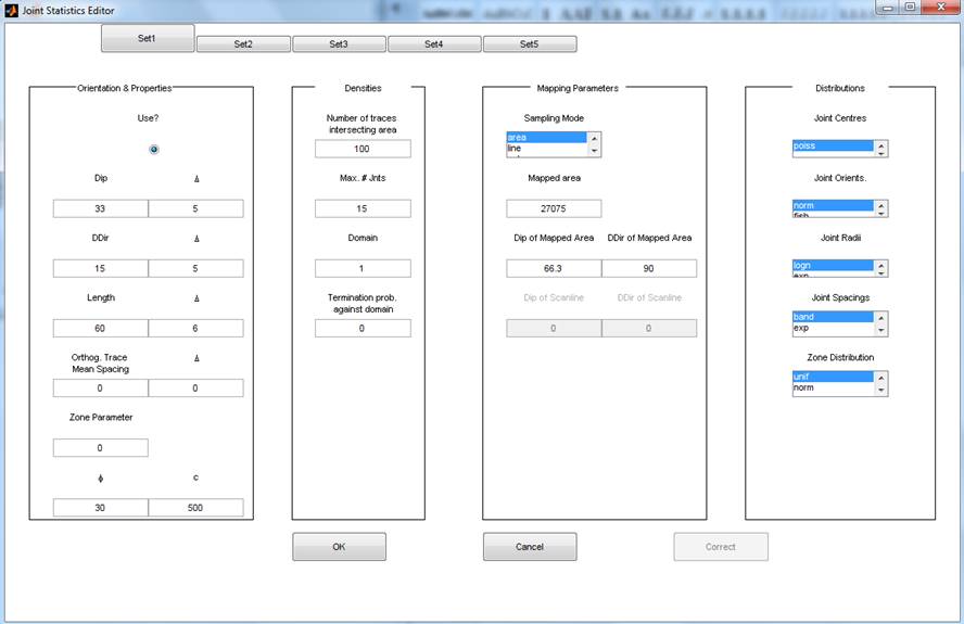
Figure 30 The joint-set
editor

If these parameters are saved to file
(using Save ‘
OPS parameters ‘
Joints), the current file format can be
inspected ‘ note that it is no longer tab delimited (see Figure 31 for
an example). As stated in Edit ‘
Beds, no
backwards compatibility for importation of OPS parameter files is guaranteed
and the import/export facility is provided strictly for use with the current
version of OPS.

 

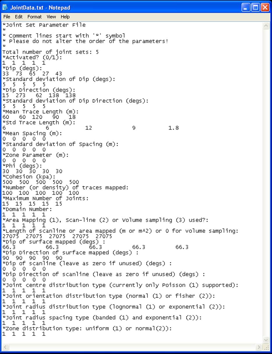
Figure 31 An example of the
file format used for the joint set parameters

Deterministic Joints ‘ edit some properties
associated with deterministic joints that have been imported (via File
‘
Load ‘
Joints‘
Deterministic Joint Polygons). Aside from the
friction angle and cohesion properties, the user can assign some uncertainties
to the location, orientation and sizes of these structures. This can be used to
represent measurement uncertainty or for general sensitivity analyses.

Clone ‘ allows the user to select a
previously defined bed or fault as a ‘seed’ for cloning (i.e. replication) in
the current model. In this way, a set of beds with a desired spacing can be
generated. Beware the generation of multiple versions of the same discontinuity
plane. Although some checking is performed, not all instances might be detected
resulting in a failure of the block modelling algorithm.

Clear Water Table ‘ remove the water table from the model.

Voids ‘  remove selected voids from the model. For UG
module only, creation of user-defined voids is also supported. The user can
specify the void dimensions and section type either manually or using the UI
tools (Figure 32). To
create a void:

1.
Select ‘Create Void’

2.
Maximimise the OPS window to facilitate visualisation of the model

3.
Click on the arrow in the
toolbar to reorient the model if necessary

4.
When ready to translate or
resize the void, click on the arrow again

5.
Click on the move tool icon in
the toolbar to move the void along the selected axis (highlights when you hover
the mouse over it)

6.
Click on the scale tool icon in
the toolbar to change the size of the void along the selected axis

7.
You can also directly edit all
parameters using the dialog box in the lower left corner of the window

8.
Click OK when complete  

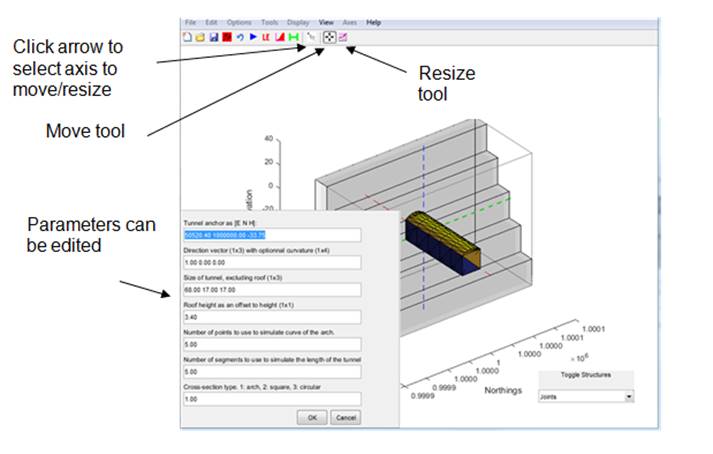
Figure 32 The UI tool for
creating a user-defined void

Domains ‘ Edit the properties associated
with each domain or delete domains. The mean rock density and the pore pressure
coefficient can be edited. The latter represents a coefficient to alter the
significance of pore pressures in a particular domain. Therefore, the values
for the coefficient can range from 0 to 1 where 0 represents no pore pressure
effects and 1 represents the full pore pressure.

 

3.1.3
Undo Menu

This
functionality allows you to undo the most recently executed editing function.
It does not include the ability to undo simulation runs.

3.1.4
Options Menu

The Options
menu is used to control the parameters used in the simulation. The first set of
options corresponds to options relating to the construction of the block model
itself. The second set (those below the separator line in the menu) correspond
specifically to the limit equilibrium analysis. As such, modifying these
options only affects the LE analysis and there is no need to recreate a block
model.

Enforce Termination Precedence ‘ will generate a dialog box allowing you to
specify truncation precedence ordering of discontinuities. Precedence is
enforced in a relational sense by specifying the set with precedence which
causes the other set to terminate. Multiple relations can be specified using
the ‘Add’ button. Termination probabilities can be specified to enforce these
relationships in a statistical rather than deterministic sense. For example,
termination of one set against another will occur:

100% of the
time if the termination probability is set to 1 (the default)

50% of the
time if the termination probability for set 1 is set to 0.5

Previous
versions of OPS did not allow the user to specify preferential termination
directions, and simply retained the portion of the terminated fracture
containing more vertices. However, you can now specify the preferred direction
for the remaining portion of the terminated discontinuity to be retained in
terms of the normal direction of the higher precedence discontinuity.

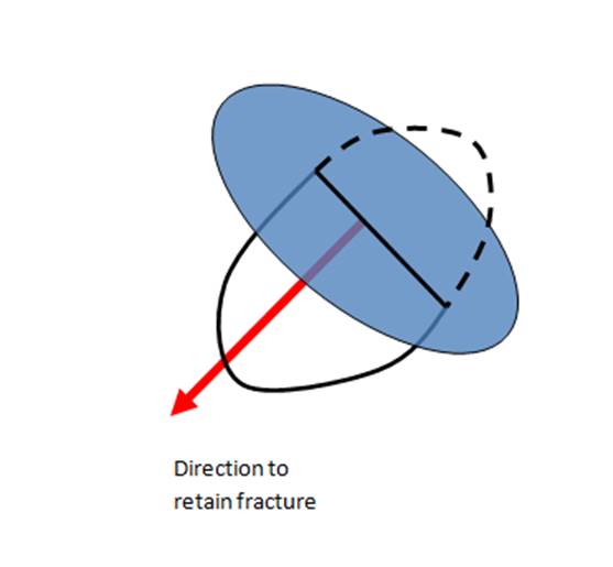
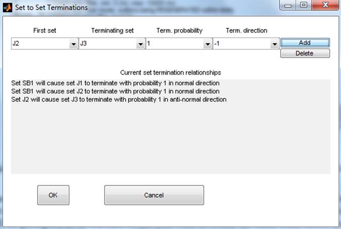
Figure 33 Example of portion of terminated discontinuity being retained and
(right) dialog box to specify termination precedence relationships.

 

Use existing joints ‘ this will force
OPS to use the existing stochastic and/or deterministic joints realised in the last
simulation for the current simulation (i.e. rather than generating a new
realisation based on the current joint set parameters). The reference to
deterministic joints applies if you have applied uncertainties to properties of
these structures (via Edit ‘
Joints ‘
Edit Deterministic Joints). Note that you will be prompted as to whether or not you wish to
retain the same scale factor (sizing) for these joints. Rescaling the joints is
a good way to perform a ‘sensitivity analysis’. For example, if increasing the
scale slightly (e.g. specify a scale factor of 1.2 for a 20% increase)
dramatically increases the number of blocks in the model, then the chances of
‘rock bridges’ being present in the original block model are high. Leave the
scale factor set to 1 for no change. Further, you will be prompted for
modifications to the spacings, dips or dip directions of the existing joints.
The ability to apply the same changes to deterministic joints is also provided,
but this will alter the representation of the deterministic joints based on the
current settings in Options ‘
Joint Representation.

Joint representation ‘ choose
number of sides for polygonal representation of the stochastic joints. All
discontinuities in OPS are triangulated therefore the hexagonal representation
of joints will attract a computational penalty of 4 times compared to a
triangular representation. Note that any joint representations, the vertices
are defined along the circle with specified radius (see Figure 34). To maintain the same area as an ideal circular disk (at the
expense of spatial extent), the area/radius of the polygon would need to be
rescaled accordingly. For triangles, squares and hexagons, this corresponds to
an increased radius of 1.6, 1.3 and 1.1 respectively. Select the menu item Randomised
rotations randomly rotate each
joint about its normal axis. In this way,
geometrical biases introduced by the polygonal representation can be reduced.

 

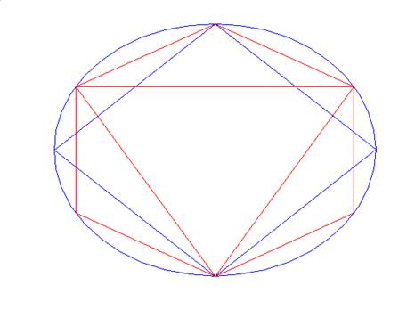
Figure 34 Triangle, square
and hexagon joint representations defined on the circle of specified radius

Filters ‘ a number of filters are
described below.

Set joint size filter ‘ set the smallest
and largest joint radii (m) to retain for stochastically generated joints. A
third argument allows you to choose whether to regenerate outliers within the
requested limits (Figure 34) or to reject them entirely.

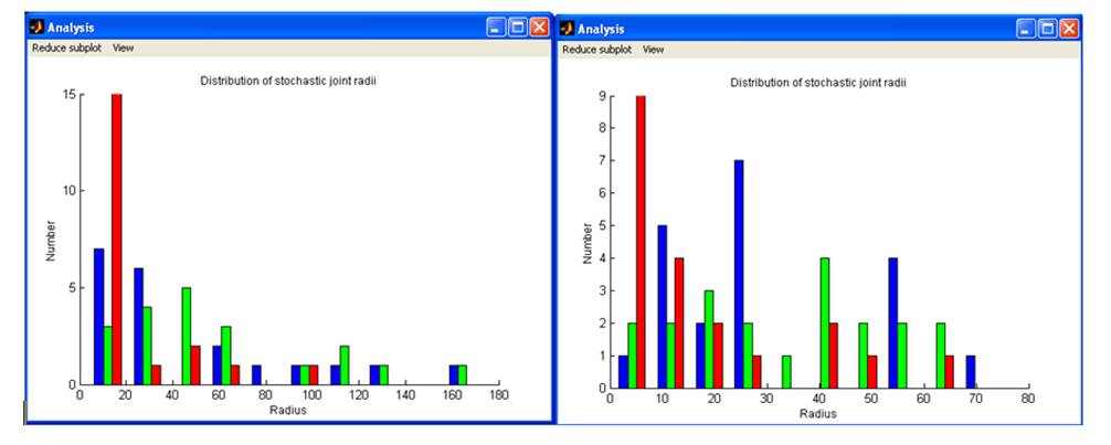
Figure 35 An example of joint
radii distributions for 3 joint sets, blue, green & red – without filtering
(left) and with joint radii greater than 80m filtered (right).

Set minimum area filter ‘ if you wish to
reject from the simulation discontinuities with areas below a certain
threshold, use this option.

Set minimum block volume ‘ set the smallest block volume (m3) to retain in the block model.
Any blocks smaller than this will be merged with their neighbours.

Set active depth ‘ the user can define a
depth below the fitted surface for which to activate joints (i.e. all other
joints will be ignored). Currently only uses a plane projected back from the
exposed surface data of the pit model to delineate the active depth. This
feature can be useful if one initially wishes to concentrate the modelling to
the exposed pit surface, and therefore reduce simulation times (see Figure 36).

Set coplanarity filter ‘ the user can
define orientation and separation thresholds to reduce the complexity of the DFN
(on a set by set basis). These thresholds are used to compare similar joints
that can be removed. Optionally, the user can also specify a direction vector
to consider the separation parameter (useful if generated joints lie
predominantly along a line such as in borehole data).

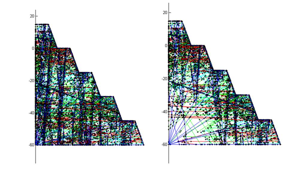
Figure 36 The result of using
the active depth feature for a complex model. The left figure shows the
intersection vertices (hence a measure of the discontinuity density) for a
reasonably complex model (4600 blocks). The right figure shows result of using
an active depth of 20 m (but using the same joint realisation as the top
figure). One can see that structures deeper than the active depth have been
discarded in this simulation and this model resulted in only 2200 blocks.

Simulation mode options ‘ you can choose
between performing a full simulation by choosing ‘Calculate Block Model’ or to
terminate the simulation early using ‘Only calculate discontinuities’. The
latter is useful for large, complex projects if one wishes to quickly examine
the network of truncated discontinuities formed in a simulation before
proceeding with a full block model.

Stochastic joint conditioning ‘ It may be
desirable to prevent stochastically generated joints from ‘daylighting’
(intersect the exposed surface) or oppositely, to only include stochastic
joints which daylight. The former can be useful if one has imported
deterministic structures such as joints observed at an outcrop (see File
‘
Load ‘
Joints ‘
Deterministic Joint Polygons). Such structures
may represent the observed sample of the population of unobserved joints within
the rock mass. If these mapped structures were used to derive the joint set statistics
used to generate the stochastic joints, then it may be desirable to ensure
there are no stochastic joints generated at the surface. In this way, the
structures intersecting the exposed surface of the model will be limited to
those which closely agree with what has been mapped in the field (Figure
37) and the structures internal to the model will
be randomly generated. This form of ‘conditioning’ is not statistically based
at this stage. The opposite option is to only include daylighting joints in the
analysis. This may be desirable if one wishes to compare the predictions of
Siromodel with a more traditional analysis method or if one deems that only a
surface based analysis is necessary. Choose between ‘None’ (no conditioning
applied), ‘Non-daylighting only’ or ‘Daylighting only’.

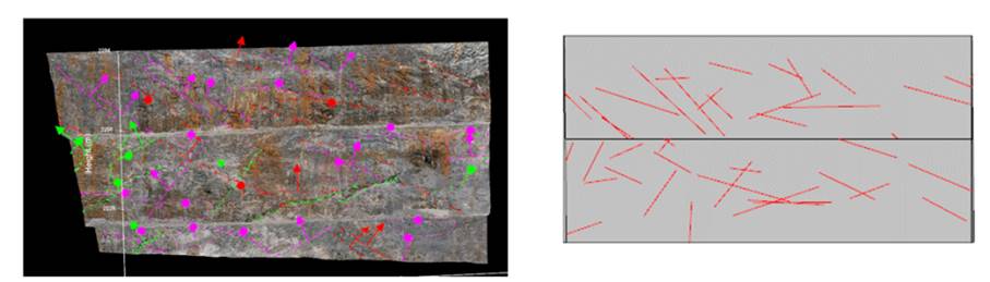
Figure 37 Structures mapped
using Sirovision (left) and exported as a Sirovision Discontinuity file. These
structures were then imported into Siromodel as polygons and surface traces
have been displayed (right). By setting the Surface condition filter, randomly
generated structures will largely not intersect the exposed surface and
therefore the resemblance with field observations will be maintained.

The remaining options correspond to the
limit equilibrium analysis. Therefore, altering these options does not require
a new block model to be constructed, but rather for the limit equilibrium
analysis to be re-run (Tools ‘
Run LE Analysis).

Ignore blocks connected to bounding surfaces ‘ activate this switch if blocks
attached to the bounding surfaces of the model are not relevant to the
analysis. Some performance improvement may be seen for projects involving large
DFN.

Specify default rock density ‘ default rock density to use in kg/m³. This value will not
apply to rock enclosed within a domain (for which a separate rock density is
specified).

Specify Static Force ‘ a static force (e.g. seismic) can be specified in terms of a
proportion of the acceleration due to gravity (g). The option of specifying a
fixed direction for this force or allowing it to act along the sliding
direction of removable blocks is also accommodated.

Set FOS cut-off for unstable (Type 1) blocks ‘ default is FOS equal to 1.

Set bolting parameters ‘ specify
parameters for use in the bolting analysis provided in the Block Visualiser,
including factor of safety, ultimate capacity and bolting modes. For the
latter, two methods are currently supported. The first allows generation of 1
bolt per block and uses all of the block’s exposed faces to determine the
location (area ‘weighted centroid of faces) and the orientation (area-weighted
mean) of the bolt. The second mode allows generation of 1 bolt for every unique
exposed face orientation (i.e. multiple bolts per block). In future, support
for importing bolt patterns generated outside of OPS will also be provided.

Set
standard deviation for phi and cohesion ‘ specify a percentage standard deviation to
apply to these parameters for a multi-carlo
simulation. Upon each simulation, the nomical
friction angle and cohesions values for the structures will be modified using
normal distributions with the specified standard deviations (defaults to 10% of
the requested phi and cohesion values for each discontinuity set). A
correlation between these two parameters can also be specified (ranging from -1
to 1, where 0 means no correlation).

LE Analysis mode ‘ this allows you to choose between a standard
limit equilibrium analysis which examines only the day-lighting blocks (surface
blocks) for stability or a ‘progressive failure’ analysis. In the latter case,
the user must specify how many iterations the software is to perform to search
for non day-lighting removable blocks. Each iteration
involves ‘peeling’ away the current layer of Type I removable blocks revealing
a new, exposed surface to be used in the limit equilibrium analysis. . Type 2
and 3 blocks from previous iterations will also be reassessed given the newly
exposed surface. This is not a stress-based analysis and the failure modes
determined for blocks may vary depending on the order in which their
surrounding blocks are removed. Note that versions older than OPS 3.0 removed
all removable block types (Types I, II & III) upon each iteration yielding
very conservative scenario.

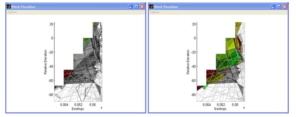
Figure 38 A comparison of a standard LE analysis (left) with a progressive
failure analysis (right). The model is being viewed from the side. Blocks bound
to the non-release surfaces have been toggled off for clarity.

3.1.5    Tools Menu

The Tools
menu is used to run the simulation and study the results.

Run simulation ‘ this will prompt you as
to how many you wish to run (note that the ‘Run multiple projects’ option, present
in OPS version 1.0 and earlier, can now be accessed via File
‘
Load ‘
Rerun full simulations for multiple projects). In
each case, the simulation/s will be performed (including block model/s creation
and LE analysis/analyses if the default Simulation mode
option is used)
and the output project files saved.

The
simulation usually consists of the following stages:

1.     DFN generator generates the joint
realisation and enforces termination precedence if requested. If the user has
selected ‘Only calculate discontinuities‘ in Options ‘
Simulation mode options, then the simulation will halt at this point.

2.     Calculate the intersections of all
polygons within the model.

3.     Calculate the blocks that form as a
result of these truncated polygons.

4.     Perform a limit equilibrium
analysis.

Run LE analysis  ‘  if a simulation has been performed, rerun the
LE analysis. This is useful if the user wishes to ‘tweak’ either the f or c properties of one or more discontinuities after a block model
has already been created. Further, one can alter domain properties (such as
rock density and pore pressure coefficient) or the position of the water table
and then quickly rerun the LE analysis. Note, however, that changes to any
geometrical properties (such as orientation or persistence) or changes to the
number of active discontinuities will not be automatically incorporated in the
existing block model (since such changes would alter the block model itself)
and so in these circumstances, a new simulation should be run.

Block Visualiser ‘ this will generate a window allowing you to
examine blocks individually or as an ensemble. Removable blocks are classified
using the Goodman & Shi criteria and are colour coded as red for Type I
(Unstable), yellow for Type II (Stable with friction) and green for Type III
(Stable without friction). Blocks susceptible to toppling have their edges
shown in white. Two sets of controls are in the lower right corner. Those
labelled ‘PFI’ allow visualisation of blocks associated different with
iterations of a progressive failure analysis. The other set highlights blocks
intersected by an interactive cross-section.

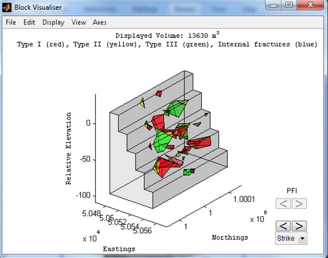
Figure 39 The ‘Block
Visualiser’ window

Toppling susceptibility is assessed using a simple geometric test.
If the weight vector of any block intersects any of the block’s exposed faces,
the block is deemed to be susceptible to toppling.

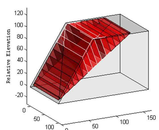
Figure 40 Blocks susceptible to toppling with edges shown in white.

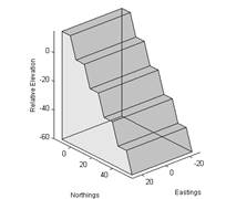
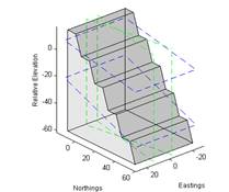
Analysis Window ‘ this will regenerate the Analysis window. This window presents data
on the deterministic and stochastic joint properties as well as a 3D
visualisation of their geometry. The colour scheme used in the 3D visualisation
is the same as that in the histograms (e.g. set 1 discontinuities blue, set 2 greeen etc). Discontintuity types
plotted in the following order ‘ beds, faults and finally stochastic and
deterministic joints. The Options menu provides the ability to truncate the
joints against the bounding volume or display some properties on the current
DFN realisation, including P32 fracture intensity statistics (defined as
fracture area per unit volume or m²/m³). Right click in the
lower left histogram to display poles or dip vectors on a lower hemisphere
polar stereonet.

 

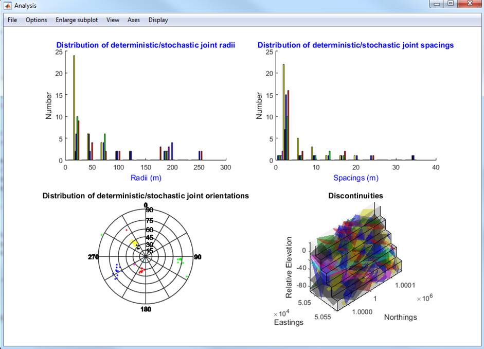
Figure 41 The ‘Analysis’ window, showing stereonet at the bottom left (use
right click to generate this)

Block Model Analysis ‘ this will
initiate the ‘Block Model Analysis‘ window and allow you to perform the
same statistical analyses for the current model as discussed previously for File
‘
Load ‘
Block Model Analysis. See 3.3 for more details.

 

3.1.6
File Menu

Load

New block model analysis ‘ load
a new set of projects

 

Save

Save plot data ‘ a
generic save utility which allows you to save any numeric data associated with
the current window. Some minor formatting is performed (limited header
information) but it is left to the user for further processing in a suitable
spreadsheet.

 

 

3.1.7
Display Menu

The Display
menu is used to toggle various model properties on or off.

Toggle Bounding Volume ‘ toggle the visibility of the bounding volume.

Toggle Edges ‘
toggle the visibility of all edges.

 

3.1.8    View Menu

The View menu
is used to set a new view angle on all plot axes that are currently open.

Plan – View all axes from the positive
Relative Elevation axis with the Northings axis positioned vertically on the
screen.

North – View all axes from the positive
Northings axis with Relative Elevation positioned vertically on the screen.

East – View all axes from the positive
Eastings axis with Relative Elevation positioned vertically on the screen.

Current – View all axes from the same
position as currently used in the OPS Control window.

Strike – View all axes along the initial
strike of the pit.

Perpendicular to Strike – View all axes
along the direction perpendicular to the initial strike of the pit.

Zoom ‘ interactive zoom. Click and drag
for 2D plots or left click/right click for 3D plots. Double click to return to
the original view.

Rotate/Disable Zoom ‘ return to rotate
mode.

3.1.9    Axes Menu

The
Axes menu is used to alter the axis properties for the selected plot.

Linear
X/Y/Z ‘ set the x/y/z-axis scale of the selected
plot to linear.

Log
X/Y/Z ‘ set the x/y/z-axis scale of the selected
plot to logarithmic.

Set
X/Y/Z limits ‘
set the limits of the x/y/z-axis.

Reverse
X/Y/Z Direction ‘ reverse the direction of the
x/y/z-axis.

Freeze/automatic
axis scaling ‘ control the scaling of figure
axes.

Edit
Title ‘ modify the title of the selected plot.

Edit
X/Y/Z label ‘ modify the x/y/z-axis label of the
selected plot.

Toggle
grid ‘ toggle the presence of a
grid on the selected plot.

3.2
The Block Visualiser Window

To improve plotting efficiency, this window
now only shows Type 1 to 3 blocks by default. To show other blocks, use the
Display menu items. Note that this window now includes an interactive
cross-section generator in its bottom right hand corner (see Figure 39). Simply select the axis
perpendicular to the desired cross-section and then use the arrows.

The menus
available from this window are as follows:

3.2.1
File Menu

Load

Toggle
Overlay Surface ‘ overlay a surface on the model.

Save

Export Visible Blocks ‘
Export the blocks currently visible in the window to a DXF file. These can be
exported as either fully triangulated or polygon representations. The former
can be useful if trying to define domains within OPS. For example, to define a
domain defined between two bedding layers,

1.
Run a simulation with two
bedding layers defined.

2.
Using the Block Visualiser menu
Display ‘
Block Selector, select the block that defines
the domain.

3.
Using the Block Visualiser menu
File ‘
Save ‘
Export Visible Blocks, export the block as a
triangulated representation to a dxf file. This can now be imported into OPS as
a domain.

Statistics for Visible Blocks ‘ Save
block statistics to a text file.

Save plot data ‘ see section 4 Common functions.

 

 

3.2.2    Edit
Menu

Bolt Visible Blocks ‘ render immovable
the blocks currently visible in the window. See section 2 for
details. The tensile and shear
forces imparted on the bolt by that block alone are calculated. Bolts are
assumed to be positioned at the centre of exposed surfaces of the blocks and
oriented at 90 degrees to these surfaces.Two bolting
modes are currently supported (see description in section 3.1.4). The bolting visualisation can be toggled on
or off using the Toggle Structures drop down menu at the bottom of the window.

Unbolt Visible Blocks ‘ remove all
bolting from the currently visible blocks.

Unbolt All Blocks ‘ remove all bolting
from the analysis.

Merge Small Blocks ‘ allows the user to specify
a further round of block merging (this is also performed with ‘Run Simulation’
if the user specified Options ‘
Filters ‘
Set minimum block volume).

Define hanging wall ‘ generates a polygon
selection tool to allow the user to define the section of a void to be used in
hanging wall analyses (e.g. ELOS).

 

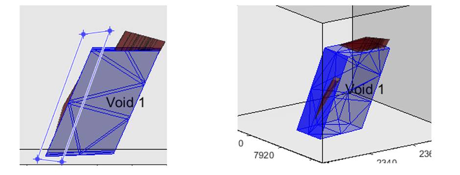
Figure 42 Polygon tool being used to select part of the void (left) to be
labelled as the hanging wall (shown in darker blue on right)

 

3.2.3    Display
Menu

Refresh ‘ regenerate the Block
Visualiser window.

Toggle Bound Blocks ‘ toggle the
visibility of blocks in contact with the bound surfaces of the model (see Figure 5).

Toggle Type 1 Blocks – toggle the
visibility of unstable blocks (red).

Toggle Type 2 Blocks – toggle the
visibility of blocks stable given the current surface properties/forces
(yellow).

Toggle Type 3 Blocks – toggle the
visibility of blocks that are geometrically stable (green).

Toggle Blocks Touching Voids – the
toggle the visibility of block daylighting on voids.

Select Blocks (mouse) ‘ ‘ enables the
user to visually select a block by clicking on it. Multiple blocks can be
selected by holding the CTRL. Validate section by pressing the Enter key or cancel the selection by
pressing Escape key. 

Note: the rotation and the zoom tool can be
used during the selection by pressing CTRL+R or CTRL+Z respectively. To return
to selection mode press the Escape
key once.

Select Blocks within a polygon (mouse) ‘
enables the user to visually select multiple blocks by drawing a polygon
overlaying the model (Figure
43). Left click to add points to the polygon.
Close the polygon by left clicking on its first vertex. At that stage the
selection polygon can be optionally refined by using the mouse to drag the
vertices. Double click inside the
polygon to validate the selection. Note that selection can be cancelled at any
time by pressing Escape key.

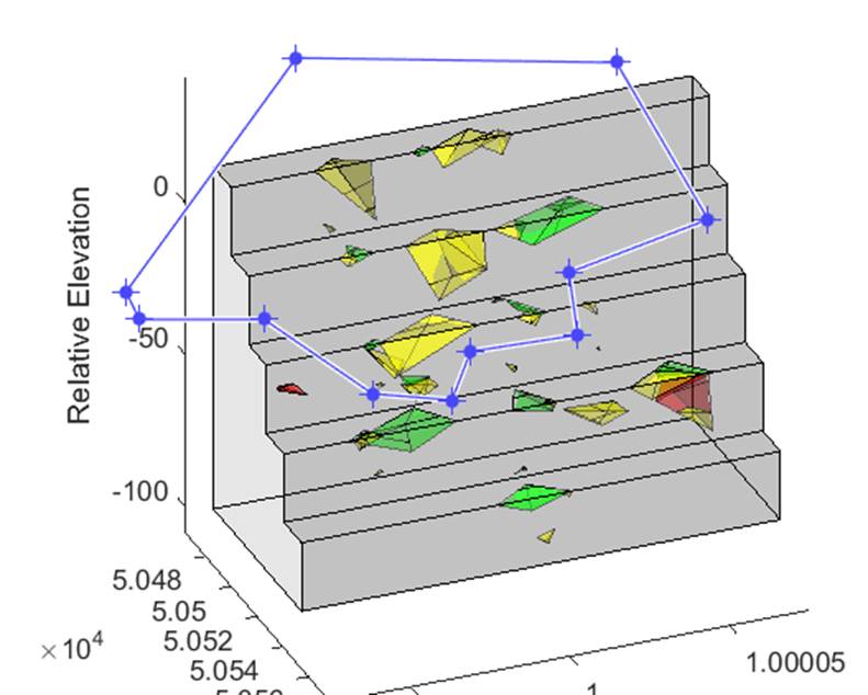
Figure 43 Select multiple blocks

Toggle Bolted Blocks – toggle the
visibility of bolted blocks.

Show Bolt Information ‘ show information
on the bolting that has been applied.This includes
bolt location, tensile and shear forces. Specification of bolt parameters such
as ultimate capacity and factor of safety cutoff
should be made using the main figure Options menu item, Options ‘
Set the FOS cutoff and
ultimate capacity for bolting.

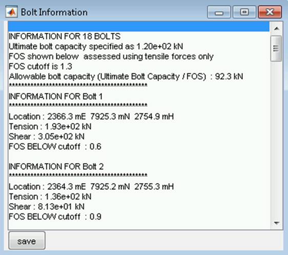
Figure 44 Bolt information dialog box showing bolt location, tensile and
shear forces

 

 

Show single bench ‘ only show the blocks
at the elevation of the specified bench. Note that large blocks may ‘belong’ to
several benches.

Show specific blocks ‘ specify the labels of blocks to show. You can use the colon
operator to specify congruent lists. For example, entering ‘2 4:6 53’ (without
the quotes) would highlight blocks 2,4,5,6 & 53.

Show information of visible blocks
‘ show block related information, including removal
force and removal vector for removable blocks.

Show dilution information using visible blocks
‘ show dilution information using the blocks
currently visible in the Block Visulaliser. Also
calculates ELOS (Equivalent linear overbreak/slough) if a hanging wall has been
defined (see Block Visualiser function Edit ‘
Define hanging wall) and a similar measure for the
total void surface (the term ‘Total skin’ has been used in this case). More
details about the calculations are presented in the description of the Block
Model Analysis function ‘Overbreak and dilution estimation’. Note that it is
left to the user to ensure that the blocks selected are appropriate for the
particular analysis being performed (e.g. hanging wall versus stope back).

 

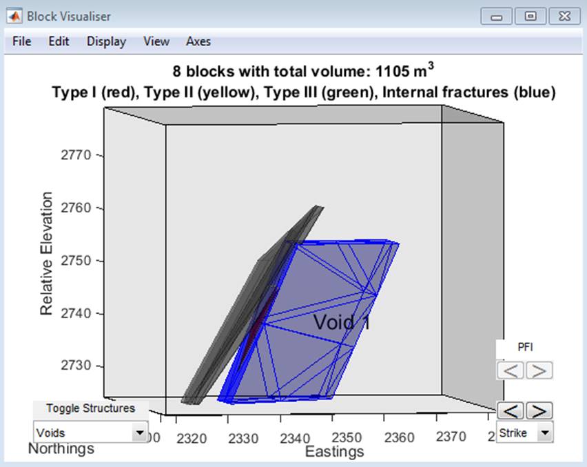
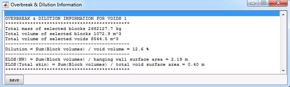
Figure 45 Dialog box showing dilution information for the blocks shown in the
top figure

 

Cycle through blocks ‘ the Visualiser will toggle the visibility of all blocks in the
block model.

Toggle Bounding Volume ‘ toggle the visibility of the bounding volume.

Toggle Wire Frame ‘ toggle the visibility of the wire frame of the bounding volume.
Note that the term ‘wire frame’ refers solely to the edges of the triangulation
of the bounding volume. Since blocks located on the boundaries of the bounding
volume also contain these edges, one may not notice any change if all these
blocks are being visualised (see ‘Toggle Edges’).

Toggle Edges ‘
toggle the visibility of all block edges. This will not toggle the bounding
volume’s ‘wire frame’.

Toggle Fractures ‘ toggle the visibility of all
intra-block fractures (blue polygons). These are fractures that reside inside
blocks and are partially through-going (hence they do not contribute to the
formation of blocks). Note that by definition, it is impossible for a fracture
to reside in more than one block.

Figure 46 Intra-block fractures (blue polygons) shown inside their ‘parent
blocks’ (left) and in isolation (right)

Block Animator ‘
animate the removable blocks. The animation is based on the calculated removal
vector of the block. Blocks with upwards removal vectors are also animated
(either due to kinematic feasibility or due to external forces). Note that this
animation is purely for visualising the forces at work and does not represent
real trajectories. For a more accurate representation of block trajectories
upon sliding, please see the bench retention analysis tool in 3.3.3.

Exploded View ‘ show the currently
visible blocks slightly separated. Specify the maximum distance to shift the
outer most blocks (distance shifted is proportional to the block’s distance
from the centroid of the model).

Block Selector ‘
generate the Block selector window (known as the BlockStats
window in previous versions). This will show some statistics for the blocks
currently visible, such as volume, surface area, number of intra-block
fractures, and for removable blocks, the factor of safety, removal vector dip
and dip direction. The user can click on the row corresponding to a particular
block and that block alone will be displayed. Note that clicking on the top
(title) row will allow the user to sort the list of blocks (see Figure 47).

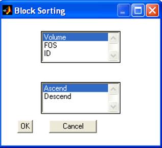
Figure 47 The options available
when sorting the list of displayed blocks.

3.3      The
Block Model Analysis Window

 

The Block Model Analysis Window is allows
the user to analyse one or multiple projects. By default, no blocks are
filtered from the analysis at the start of a block model analysis. The user
must use the Edit menu within the Block Model Analysis window to restrict the
analysis to specific block types. Unless otherwise stated, the stability
related analysis functions available under the Options menu will use
all removable blocks in their calculations. This can be controlled using the Edit
menu. For example, if only Type 1 removable blocks are of interest, then Edit
‘
Filter data based on FOS can be used to enforce
this filter. However, one should be aware that the applied filter will be based
on the block properties at the time of filtering and will
not take into account changing block properties that may result from an
analysis. For example, a pushback analysis (Options ‘
Push-back analysis) takes the current
exposed surface, shifts it into the rock mass and excavates rock behind the
surface. A limit-equilibrium stability analysis is then performed for this new
exposure and the results reported. However, if the user had applied a filter
prior to this analysis that excluded these blocks, then no blocks would be
considered in the new exposure. Note that if a Progressive failure analysis was
performed on the project data prior to initiating a Block Model Analysis, then
this issue would not arise.

The menus
available from this window are as follows:

3.3.1
File
Menu

Load

New Block Model Analysis ‘ load multiple project (*.opp) files or a block
model analysis (*.opa) file.

Toggle Overlay Surface ‘ overlay a surface (only available for Hazard Maps).

Save

Current Block Model Analysis ‘ save a current block model analysis file (*.opa)
file. 

Save Plot Data ‘ see section 4 Common functions.

Save Raw Data ‘ a generic save utility which allows you to save any numeric raw
data arrays associated with current plot. No formatting is performed and data
is written out in ascii format. The standard format is such that each data row
corresponds to an individual project and each data column to a block parameter
(e.g. size), however this may vary depending on the data type (e.g. spatial data
written out as 3-column format). Multiple data files may be written with file
names corresponding to the parameter. See individual Options to determine which
data can be saved with this facility.

Block Statistics
‘ allows you to save the block statistics for
each project loaded into the Block Model Analysis Window. A separate statistics
file is created for each one. To create a single file, first apply Edit
‘
Concatenate all data into a single data set.

3.3.2
Edit Menu

Provides
access to several filters to allow you to limit the block model analysis to a
subset of data. Note that filters are applied in a cumulative sense (e.g. first
applying a volume filter to limit volumes to 0 to 1000m3 followed by the
application of a factor of safety filter to limit the analysis to blocks with a
FOS between 0 and 1 will result in ‘Blocks with volumes less than 1000m3 and
FOS less than 1 being considered). To review the filters that have been
applied, use Options
‘ Processing info.

Add projects ‘ Add new projects for the analysis.

Reorder projects ‘ Change the order in which projects are stored.

Concatenate all
data into a single data set ‘ multiple projects
are combined. This filter is not reversible (i.e. one needs to start a new
block model analysis to reset this).

Filter selected
projects ‘ exclude data from selected projects
from the analysis.

Filter data based
on volumes
‘ allows the user to specify a minimum and
maximum block volume to be analysed.

Filter data based
on FOS
‘ allows the user to specify the minimum and
maximum factor of safety of a block to be included in the analysis.

Filter data based
on bench number
‘ allows the user to specify a single bench
number to be analysed.

Filter blocks
bound to non-release surfaces ‘ exclude
blocks that are bound to non-release surfaces (i.e. back, base and sides of a
user defined model).

Filter removable
blocks ‘
exclude removable blocks from the analysis.

Specify volume of
interest ‘
exclude blocks outside a specified volume of
interest. This tool allows the user to visually define a domain represented as
an axis aligned box or an oriented box. Upon selecting the tool,

1.
the user can choose to use the
OPS main window or the block visualiser window (if open).

2.
Maximimise the OPS window to facilitate visualisation of the model

3.
Click on the arrow in the
toolbar to reorient the model if necessary

4.
When ready to translate or
resize the volume of interest, click on the arrow again

5.
Click on the move tool icon in
the toolbar to move the box along the selected axis (highlights when you hover
the mouse over it)

6.
Click on the scale tool icon in
the toolbar to change the size of the box along the selected axis

7.
You can also directly edit all
parameters using the dialog box in the lower left corner of the window

8.
Click OK when complete  

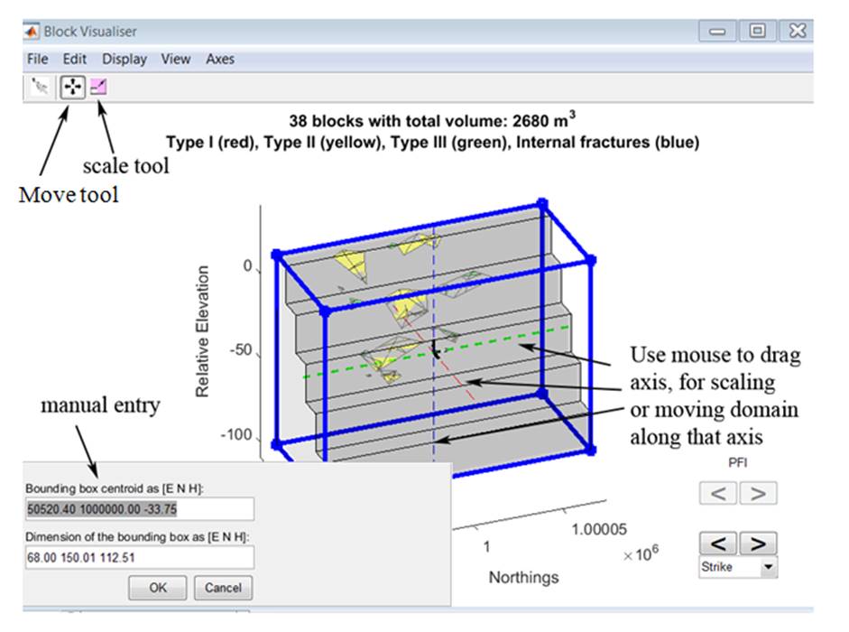
Figure 48 Interactively defining domain

Filter blocks not
in contact with voids
‘ exclude any blocks not directly in contact
(i.e. daylighting) with voids.

Remove Filter/s ‘ Removes the filter values (except for Concatenate all data into a
single data set).

3.3.3    Options Menu

Block Numbers ‘ the histogram of total
block numbers for the projects being analysed will be presented.

Block Volumes ‘ the distribution of
block volumes will be presented graphically. Right click on the centre graph
for more options. The File ‘
Save ‘
Save raw data menu can
be used to save volume data.

Block Positions ‘ allows the user to
analyse the distribution of block centroids along a specified direction. This
could be useful for analysis along the strike direction of an open cut wall or
along the elevation of an underground shaft.

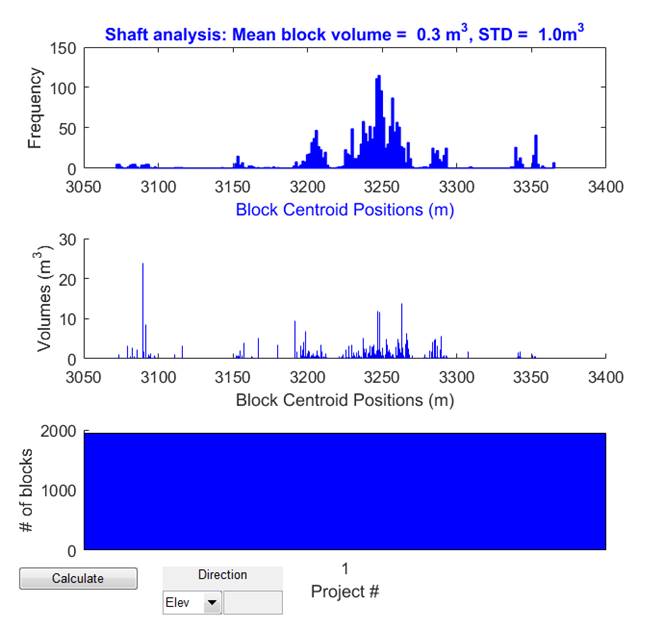
Figure 49
Example of a block position analysis performed along the elevation of an
underground shaft

 

Overbreak & Dilution estimation ‘
(UG module only) shows estimation of the volume, mass and overbreak/dilution
percentage for each project. Uses void data present in the first project
(assumes all projects contain same void geometry). The overbreak or dilution
percentage is calculated using the following formula:

For projects with multiple voids, user is
prompted as to which voids to consider in the analysis.

The ELOS (Equivalent linear
overbreak/slough) is calculated using the following formula:

This definition has been described and
illustrated in Oddie & Pascoe (2005) and is shown
in Figure 50.

 

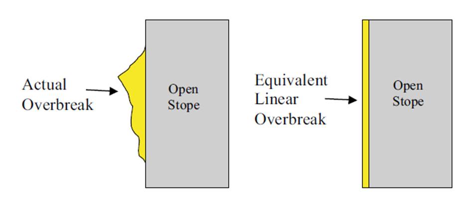
Figure 50 Schematic
representation of ELOS (taken from Fig 3 of Oddie
& Pascoe, 2005).

 

Once again, for projects with multiple
voids, user is prompted as to which voids to consider in the analysis. Since
ELOS should only be applied to a specified section of the void (e.g. hanging
wall of the stope), the user should ensure that the hanging wall has been
defined for at least the first project used in this analysis. The user can also
modify the area used in the analysis using the edit box in the lower left
corner. As with all Block Model Analysis functions, appropriate filtering
should be applied so that only blocks relevant to the analysis are consdired. For example, for hanging wall analysis, use the Edit-Filter blocks not in contact with
voids , Edit-Filter blocks bound to non-release surfaces and then
Edit-Specify volume of interest). Then select Tools – Update Block Visualiser to show which blocks are currently selected.

 

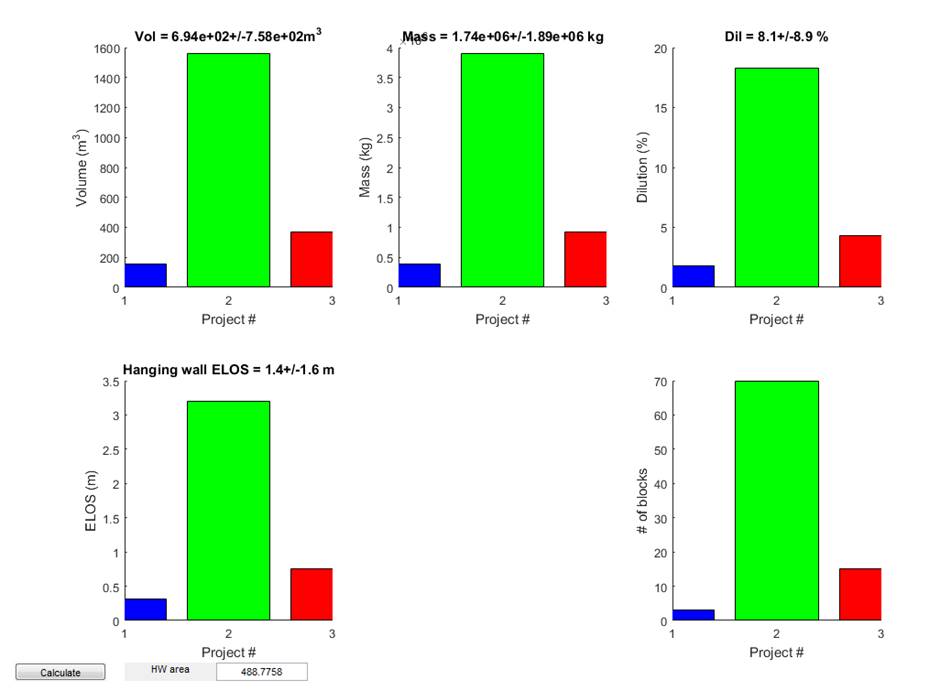
Figure 51 Overbreak and Dilution estimation for 3 projects.

Voussoir beam analysis ‘ (UG module only) applies a Voussoir
laminated beam analysis. Uses void data present in the first project (assumes
all projects contain same void geometry). The method defined by Diederichs & Kaiser (1999) is used. The method deals
with thin laminations (span-to-thickness ratio greater than 10) under the
influence of self-weight or moderate surcharge loading. Therefore, only
crushing and snap-through failure are hereafter considered. Sliding stability
is included in the analyses but does not control limiting dimensions for thin
beams.

The mid-span deflection and buckling limit
(percentage of beam thicknesses tested for which no stable solution exists) and
mid-span deflection. Assumptions and limitations in this method described by
the authors include: 

‘
lamination thickness is known
and where the modulus can be estimated with some degree of reliability

‘
not recommended for very large
spans (>100 m for steeply inclined spans and >60 m for horizontal spans)

‘
consistent excavation quality
is also assumed. Over-blasting, or uneven excavation surface geometry will
negatively impact roof stability.

‘
joints are assumed to be rough
enough to provide frictional resistance under low to moderate confinement

‘
the span to thickness ratios
are greater than 10.

‘
sliding failure along joints at
the abutments or within the beam is not considered.

‘
it is assumed that there is no
frictional or cohesive resistance along the interfaces between the laminations.
This represents a worst case assumption since such resistance increases the
stability of the beams.

‘
no low to mid angle jointing is
present.

‘
this method is not suitable for
poor rockmasses with a low RQD rating (<50) and
more than three joints sets.

‘
only the first (lowermost)
lamination is considered and not a composite beam structure. This is based on
the assumption that, provided the beam thickness is stability of the whole roof
is controlled by the stability of this first beam.

‘
the influence of the gravity
load component parallel to inclined laminations is ignored.

 

To use this function, filter out blocks
that are not relevant to the analysis (e.g. for hanging wall analysis, use the Edit-Filter blocks not in contact with
voids , Edit-Filter blocks bound to non-release surfaces and then
Edit-Specify volume of interest). Then select Tools – Update Block Visualiser to show which blocks are currently selected. An example is shown
below.

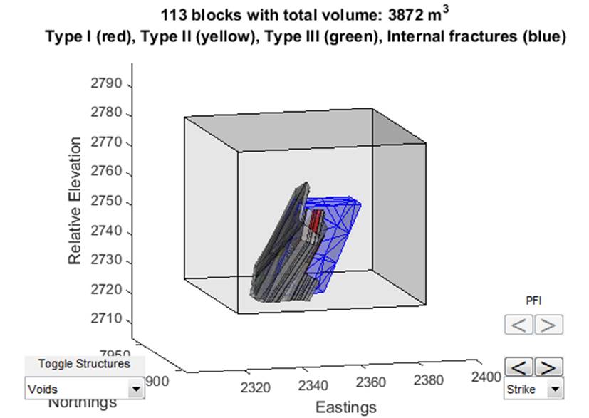
Figure 52 Example of excluding blocks not needed in the analysis

Then use the Voussoir beam analysis tool to set the parameters required
for the analysis. The parameters include:

‘
Friction angle to use to assess
the factor of safety for sliding failure

‘
Lamination dip

‘
Support pressure (currently
assumed to be zero)

‘
Young’s modulus values to test

‘
Minimum and maximum lamination
thicknesses to test

‘
UCS value, adjusted for the
rock mass conditions. Diederichs & Kaiser (1999)
suggest reduction by one third to one half of lab values.

‘
Yield criteria as a buckling
limit % (used in determining the maximum allowable span)

The plots
produced are shown in Figure 53. They
include:

‘
Midspan deflection as a
function of beam thickness

‘
Buckling limit as a function of
beam thickness

‘
Maximum allowable span as a
function of beam thickness (based on a buckling limit criteria)

‘
Factor of safety (for both
sliding and crush failure) as a function of thickness

Two beam models
are assessed for all calculations, the infinite beam model (2D approximation)
and the square beam model. Plots are shown on the same axes to allow
interpolation.

If multiple
projects are being analysed, you can control whether span estimations from each
of the projects are used or a user specified value is desired. Simply type the
maximum span value in the edit box to do this.

Right click on
the plots to access toggling functions.

 

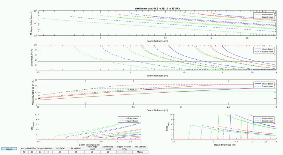
Figure 53 Voussoir
beam analysis for 3 projects.

 

Block Shapes ‘ the distribution of maximum block sizes and shapes will be presented
graphically. Right click on the centre graph for more options. Note that
several indices characterising shape are provided. The shape index γ is
defined as the ratio of the block volume V to that of a sphere with diameter
equals the maximum block size, lmax (see Wang et. al.
2003)

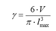
The shape
indices α and β are an alternate description of block shape as
described in Kalenchuk et. al. (2006). For a block
with surface area As and volume V, these are derived using the inter-vertex
vectors (face edges, diagonals  and
internal diagonals) formed from all vertex pairs, rejecting vectors with
lengths less than the median value, calculating the average length lavg and using combinatorial pairs of vectors (i.e. a and b) to determine angular relationships: 

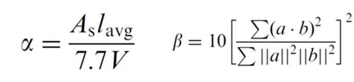
Note that
the α and β indices rely on calculations of combinations of vertices
which becomes intractable for very complex blocks (e.g. with hundreds of
vertices). Such blocks are typically representative of the unfragmented rock
mass which is rarely of interest anyway. Therefore blocks bound to non-release
surfaces are automatically excluded from the α and β calculations. They
should be excluded from the entire shape analysis using Edit
‘
Filter blocks bound to non-release surfaces.

The File
‘
Save ‘
Save raw data menu can
be used to save maximum block sizes, γ as well as α and β
indices.

Factors of safety ‘ presents the factors
of safety for all removable blocks in all projects. The File
‘
Save ‘
Save raw data menu can
be used to save this data.

It is worth mentioning the difficulties
associated with the concept of probability of failure (or PoF)
at this point. To understand these, let’s summarise the ways Siromodel can be
used, including

‘
Assess a single failure on the
slope. See the example data NewExampleProject.opp
that comes with Siromodel

‘
Assess multiple failures on the
slope. See the example BFJExample.opp that comes with
Siromodel.

 

The second mode of use is more common.

Siromodel can be used to assess a
structural model built from deterministic structures, stochastic structures, or
both.

Finally, Siromodel can be used to assess 1
simulation or the results from multiple simulations (Monte Carlo).

Due to these many modes of use, the term
‘Probability of Failure’ can be very misleading. For example, are we estimating
the ‘probability’ based on a single failure assessed multiple times or multiple
failures assessed once? Further, what do mean by failure? One of the modes
simulated in Siromodel, a combination of modes, or a mode (such as composite
failure) not simulated in Siromodel?

Therefore, we prefer for the user to assess
the fraction or percentage of occurrences for the event of interest using
Siromodel, and it is then up to them to then report this figure as appropriate.

Here is an example of how such a percentage
can be derived. The central chart in Options ‘
Factors of safety is
relevant here. Rescale the x-axis if needed using Axes ‘ LogX and
then click on that chart. Right click on the chart and select Toggle project curves and then Toggle
project labels to remove unwanted clutter. This
produces the following chart with mean and 95% confidence interval curves
shown.

Figure 54
Cumulative frequency plot of FOS for 100 simulations

So now you have the factors of safety for
all events for all projects displayed on a cumulative frequency plot. If you
set the FOS cutoff at 1.5, you can plot this line on
the chart using (Axes ‘ Add vertical line). You can now see
from this analysis that around 7% of events fall below this cutoff
if the mean curve is considered but for 95% confidence, this could be as high
as around 18% (intersection of red line and top dashed curve). Some people
might refer to this as PoF = 0.07. For the reasons
mentions above, we think this is a confusing term that doesn’t capture the
complexity and constraints of the analysis.

Removal forces ‘ presents a histogram of
the removal forces for all the removable blocks in all projects. These are
calculated as the forces inducing motion minus the forces resisting motion. The
File ‘
Save ‘
Save raw data menu can
be used to save this data.

Removal vectors ‘ presents data on the
removal (i.e. sliding) vectors. Note that the points represent the dip-vector
associated with these planes or wedges. This is in contrast to the plots
generated by OPS versions older than 1.0 (inclusive), which showed plane poles.
The File ‘
Save ‘
Save raw data menu can
be used to save dips, dip directions, block Ids and failure type data.

Failure modes ‘ for all removable
blocks, the mode of failure will be reported. Data on the number of toppling
blocks per project is presented. Also, the number of contact planes (either 1
for plane failure or 2 or more for wedge type failures) is presented. To limit
to Type I blocks, use Edit ‘
Filter data based on FOS. The File
‘
Save ‘
Save raw data menu can be used to save failure mode data.

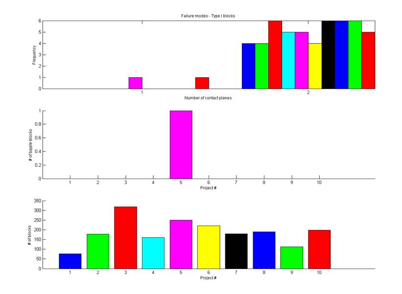
Figure 55 Failure mode analysis plots for 10 projects.

Hazard density map
‘ presents a 2D contour plot representing the density of hazard events
(removable blocks) on the excavation surface. The data is processed in discrete
bins on a projection plane, the number of which can be changed by the user.The default projection plane is a vertical plane
oriented along the strike of the excavation surface (or the bounding volume for
underground models) however the user can change this. For example, for
assessment of underground excavations, the user can select an orientation that
is consistent with the excavation geometry. The hazard events will then be
projected onto this plane.

Interpretation of this
plot is as follows. For multiple simulations, this plot represents the
probability that a simulation will generate a hazard at a particular location.
This can be thought of as the number events per bin per simulation multiplied
by 100%. Percentages greater than 100% are possible if multiple events are
recorded per bin. The hazard locations are calculated using the centroids of
the removable blocks. A 2D histogram is calculated using the locations of these
hazards onto the gridded plane. Right click on the plot to be presented with
options to change the bin size for the grid as well as the contouring.

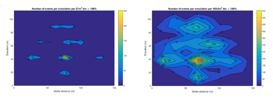
Figure 56 A hazard density map for 100 projects shown for small (left) and
large (right) bin sizes.

Hazard map ‘ presents a colour-coded
plot representing all the removable blocks on the excavation surface. The
location of the points corresponds to the mean position of the exposed vertices
of removable blocks. The size of the points is inversely proportional to the
factor of safety but limited to the range stated in the title. The File
‘
Save ‘
Save raw data menu can be used to save the locations (mean
of the exposed vertices) and factors of safety of removable blocks.

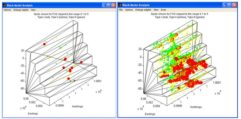
Figure 57 A Hazard map for a single project (left) and 200 projects.

Pseudo Slope Deformation ‘ OPS does not predict slope deformation as
such but rather movements in individual blocks based on limit equilibrium
analysis. However, in order to provide some guidance as to how such movements
might relate to slope deformation measurements in the field, a tool has been
developed. The deformation ‘metric’ used is the predicted sliding velocities of
the blocks. This metric is modified based on the position and resolution of the
detector. In this way, the loss of sensitivity of a detector to slope
deformation because of poor detector positioning or poor resolution can be
simulated. When requested for a detector resolution, specify in terms of
radians (not degrees). One can estimate the resolution by dividing the
footprint width or diameter by the distance to the detector. For example, if
the footprint is 5 metres when the range is 100 metres, the detector resolution
should be specified as 5/100 or 0.05 radians.

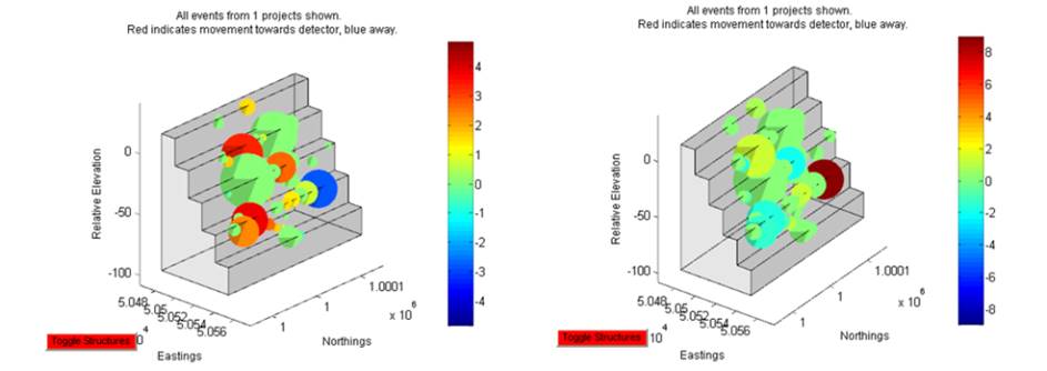
Figure 58 A Pseudo Slope deformation analysis with detector place directly in
front of the region of interest (left) and 1000m to the North. The latter
results in a significant reduction in detector sensitivity to block motions.

 

Isoplethogram ‘ A stability
isoplethogram is a means of interrogating the stability characteristics of the
internal rock mass and optimise excavation geometry accordingly (Windsor &
Thompson 1996; Elmouttie M.K., Kr’henb’hl G. & Soliman A 2016). The File
‘
Save ‘
Save raw data menu can
be used to save this data as either a 4-column ascii (storing dips, dip
directions, number of removable blocks and volumes of removable blocks) or
individual files of 2-dimensional matrices (for surface plotting).

A series of excavation planes pivoting from
one of four locations will be used: top crest, bottom toe, top rear or bottom
crest (Figure 59). A
user-specified anchor is also supported.

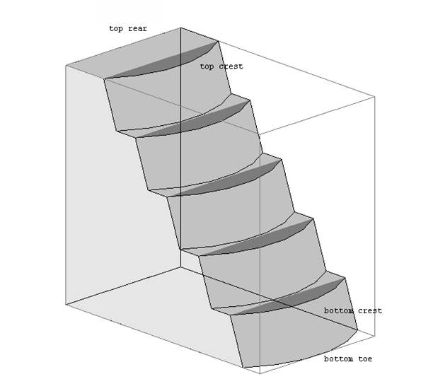
Figure 59 The four options for choosing an anchor point

For each excavation, the number and volume
of ‘daylighting’
removable blocks (kinematic analysis) will be assessed (Figure 60). Currently for plane excavations
only, the analysis also includes an estimation of newly formed polyhedra againt the proposed plane. This estimation is based on the
intra-block fractures that daylight on the proposed plane.

For the UG module, the ability to also
assess a number of orientations to apply to the current excavation void
design is also supported. In this case, the major axis of the void is
considered as the default preferred axis or the user can define this. For the
isoplethogram assessment, the specified dip and dip directions are applied to
this axis. An anchor point for these rotations must also be specified. For
example, for a proposed decline that is heading East, specifying dip directions
ranging from 70‘ to 120‘ will assess decline headings 20‘ either side of the current design.

 

 

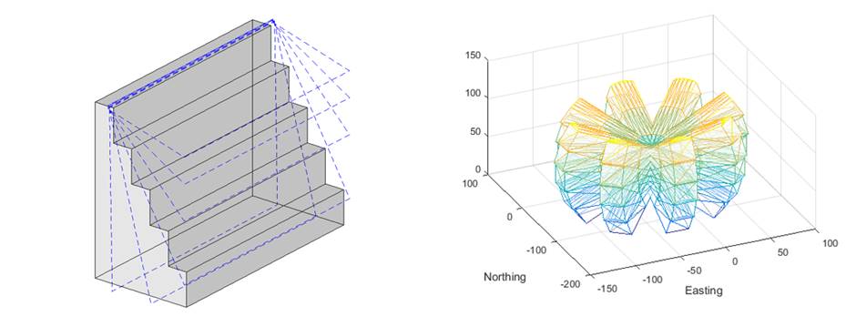
Figure
60 Left: ‘Top-crest
anchored’ excavation planes with 15 degree dip spacing (only those
corresponding to one dip direction shown for clarity). Right: For UG module
only, the ability to specify multiple orientations to orient the current void
and assess for stability. In this example, the anchor point has been specified
as the centroid of the void itself.

The user can choose the limits and the
angular spacings of dip and dip direction of the excavation planes. The
resulting graph plots dip versus dip direction of each plane with the colour
representing the number of removable blocks and this is known as a stability
isoplethogram (Figure
61). Right
click on the plot to see the available context menus to control labelling and
contouring. Click on the ‘Visualise’ button in the lower left corner of the
window to generate plots similar to those shown in Figure 60.

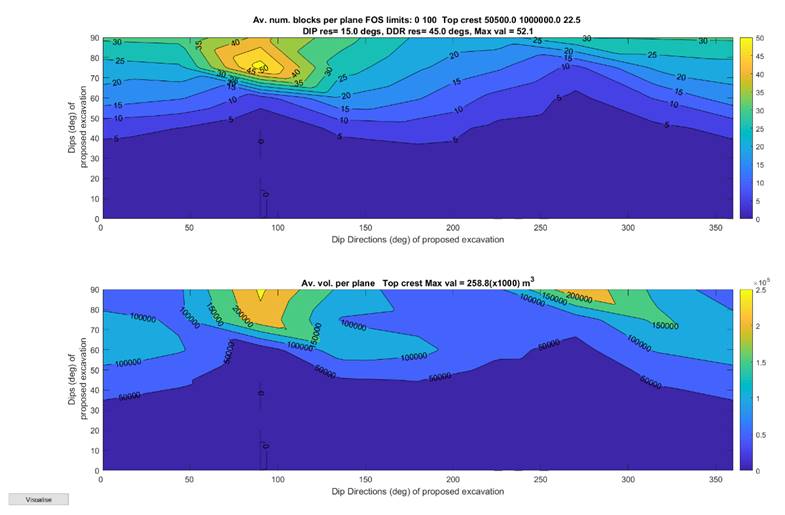
Figure 61 A stability
isoplethogram performed on BFJExample.opp using 100
DFN realisations.

Interpretation of the isoplethogram can be
explained via the use of a simple example. Consider a 100m wide cubical
bounding volume containing a solitary10m wide cube at its centre. The geometry
would appear as shown in Figure 62. This example can be considered to
be a single bench where the anchor point at the top crest is located at [50mE
0mN and 50mRE]. Only this single internal block can ever be intersected by the
excavation planes and this simplicity will assist in the interpretation of the
results.

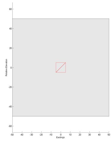
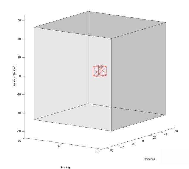
Figure 62 Simplified geometry
example used to understand isoplethograms. View along strike (left) and
isometric view (right).

As can be seen in Figure 63, the
isoplethogram for this simple geometry shows a curved pattern with a minimum
located at dip direction 270′. Due to the central location of the internal
block and the square geometry of the bounding volume, the failure at dip 45′
and dip direction 270′ is to be expected. What might be less intuitive is the
fact that the curve predicts failures at all dips greater than this. To
illustrate this, the red-dotted curve is shown which represents the ideal case
of a point-sized block located at the centre of the 100m wide bounding volume.
This curve has been generated by considering all the possible planes containing
both the top-crest anchor point as well as the centroid of the internal block.
Any excavation planes containing these points will intersect the internal block
and register a single failure in the isoplethogram. Note that if the bottom toe
had been chosen as the anchor, then due to the symmetrical geometry in this
example, the same curved feature would be present but with a minimum located at
dip direction 90′. Note that the more fine the angular spacings used for the
excavation planes, the more closely the contour plot will resemble the
theoretical red curve.

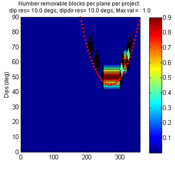
Figure 63 Top-crest anchored
isoplethogram for the geometry in Figure 62. The red dotted line shows the theoretical curve associated with
all possible planes containing both the anchor point as well as the centroid of
the 10m wide cube

Bench Retention ‘ Based on a kinematic analysis of all
removable blocks, an estimate of their impact point on the surface is made
(note that versions prior to OPS 2.0 only considered Type I blocks but now such
filtering is left to the discretion of the user). A simple collision detection
strategy is used. The default collision criterion assumes the sphere enclosing
the falling block (bounding sphere) must at least touch the bounding sphere of
a block within the rock mass. However, the user can control the collision
criterion by assigning a percentage overlap that needs to occur before a collision
is registered. Blocks are assumed to slide completely out of the wall without
rotation, and then undergo parabolic trajectories. No impact physics such as
bouncing is incorporated. No bench spillage onto lower benches is taken into
account although some account for crest loss of catch benches is taken by
excluding removable blocks from the impact calculations. The option to
introduce a swell factor is available and the ‘Failed Volume’ and ‘Spill
Widths’ charts will be updated accordingly. No account is taken of catch-bench
capacity or overfill so the values simply refer to the total spillage
accumulating at each berm. Similarly, the option to specify an ‘Angle of
Repose’ for the failed material is also available and this will update the
‘Spill Widths’ chart. These factors are incorporated using the expressions
outlined in Gibson et al. (2006, p568). Predicted block trajectories (ignoring
impact physics) are also shown using the lowest elevation block vertex as a
marker. In the case of an analysis of multiple projects, the displayed totals
(blue bars) are calculated by summing the data for all projects and dividing by
the number of projects. Maxima and mean data are calculated based on all
available data (e.g. the displayed maximum volume is the maximum observed
across all the projects).

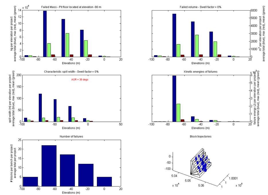
Figure 64 The bench retention charts

Pushback Analysis ‘ the user can specify the number and distance of pushback surfaces to
assess. Similar to the isoplethogram, the number of ‘daylighting’ removable (kinematic analysis) blocks
(Types I, II & III) for each pushback will be calculated. Note that the
points shown on the pushback surface/s correspond to the exposed faces of any
blocks that are ‘clipped’ by this new surface. Therefore, the plots may show
points both in front of and behind the current pushback surface/s.

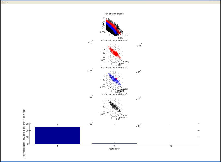
Figure 65 A pushback analysis performed using 3 pushbacks with 25 metre
spacings

Back-break Analysis ‘ the user can
specify the bench numbers to use in a back-break analysis (Ryan & Pryor
2000, see Figure 66).
This will assess for the specified benches, what the resulting back-breaks
would be given the degradation of the crest due to the presence of any
removable blocks (i.e. blocks daylighting on multiple benches are also
considered) interacting with these benches. Here, back-break is defined as the
distance away from the original crest the degraded crest moves. The maximum
back-break reported per bench is limited to the original bench width (even
though multiple bench failure can occur if the removable blocks assessed span
multiple benches).

The maximum effective face angle reported
will be equal to the face angle of the bench being investigated, and hence will
normally not be 90‘. An example is shown in Figure 67. For comparison,
the analysis is also performed using the ‘standard’ wedge type analysis, but
still based on the 3D DFN. For this analysis, processing options include
daylight vector test mode, maximum angle to classify plane failures and minimum
joint radius to consider. Crest damage is now also reported, both as total
damage per bench crest as well as individual failures.

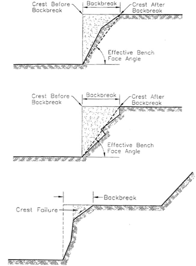
Figure 66 Definition of back
break and effective face angle (taken from Figures 3.5 & 3.6 of Ryan &
Pryor (2000))

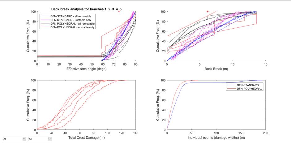
Figure 67 An example of a
back break analysis for 5 benches of 100 projects.

Probe Surface Analysis ‘ the user can define a plane or import a dxf surface to use as a
‘probe’. Blocks intersecting with this surface will be detected and the user
has the option of saving to file the identifier numbers for these blocks.
Further, the number of fractures inside each of these blocks is also reported.
This type of analysis can be useful if one has available a pre-computed failure
surface from a numerical simulation and one wishes to reconcile the block model
with this prediction. In this way, the tool serves as an indicator of the
presence of ‘rock bridges’.

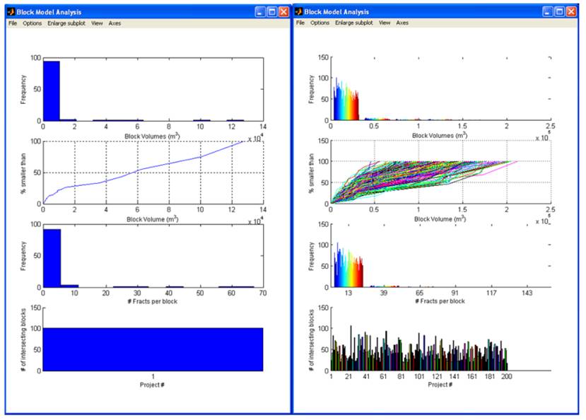
Figure 68 A probe surface analysis using the ‘BFJWaterTable.dxf‘
to probe the project BFJExample.opp (left) and 200
new realisations of this project

Fracture Statistics Analysis ‘ produces a P32 fracture intensity data cube.
If multiple projects are loaded, this represents the mean P32 values, and a P32
variance data cube is also shown.

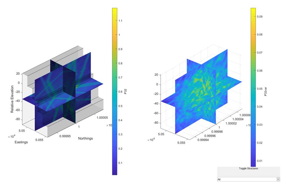
Figure 69 P32 fracture intensity (left) and variance in P32 for 100
simulations

Processing info ‘ a summary of all the
projects on which the current block model analysis is based. Note that an asterix (*) indicates several iterations of the algorithm
were needed to derive a block model. A double asterix
(**) indicates that the maximum number of iterations was reached and the block
model may not be reliable.

 

 

4       Common functions

 

Toggle Overlay Surface ‘ load a
Sirovision 3D Image or DXF triangulation to be overlayed
on the model in the OPS Control window. Select this menu again to clear the overlayed image. This option is normally only suitable if
the model itself is based on the triangulation data.

Save plot data ‘ a generic save utility
which allows you to save any numeric data associated with the current window.
Some minor formatting is performed (limited header information) but it is left
to the user for further processing in a suitable spreadsheet.

 

 

Other Hints

4.1
Filtering data for Block Model
Analyses

Any analysis conducted in a Block Model Analysis
(using a function in the Options menu) assumes that the user has excluded data
not relevant to the analysis. Failing to do so will produce non-sensical
results in the analyses. Filters that are commonly used include Edit-Filter
blocks bound to non-release surfaces to exclude blocks that
have formed against the boundary surfaces of the model and may therefore be
mis-representative in terms of size and volume, Edit-Specify
volume of interest to exclude blocks outside a
volume of interest and Edit-Filter data based on FOS to only include blocks withina range of
factor-sof safety.

4.2
Histograms

Blue text labels on
histograms indicate clickable functionality is available. Clicking the title
allows the bin number of the histogram to be changed. Clicking on the
horizontal axis label produces a figure summarising the histogram statistics.
Right click on a bar of the histogram to access a context menu. For structure
orientation histograms, right click on an empty space to access other features.

4.3
Cumulative Frequency Plots

Right click on these to
provide options to plot confidence curves. Note that such curves are only
reliable if at least 30-50 simulations have been performed. Other options
include generation of percentile plots (for Monte Carlo simulations – user
specifies the percentile of interest and the parameter value for each
simulation is shown) and showing of project labels.

4.4
DXF files

OPS supports imports and exports of dxf files
using the following entities:

‘       Polygons ‘ Polylines (AcDb3dPolyline)

‘       Triangulated surfaces (meshes) ‘ polyface meshes (AcDbPolyFaceMesh),
3DFace (AcDbFace)

4.5
General

Hold the mouse over
edit boxes, drop down lists and other similar controls to receive a tool-tips.

 

5
Worked Examples

The
following section describes two worked examples to quickly introduce the user
to the main software functionality. The example projects discussed below should
be located in the ‘Projects’ directory in the OPS installation directory (e.g.
C:\Program Files\OPS\Projects).

5.1      Simple
Example

An example project file called ‘NewExampleProject.opp‘ has been provided. Using File
‘
Load ‘
Project, select this file. ‘Click-and-drag’ in
the OPS Control window to change the view of this model. Select File
‘
Project Properties to view details about the project. Note that the PIT
MODEL information describes the type of model that has been created, in this
case a ‘linear’ (i.e. editable) model. The DISCONTINUITIES information informs
us that the only discontinuities present in this project are 2 activated beds
and 2 activated faults. The RESULTS information informs us that a simulation
has already been performed with 11 blocks detected and also reports the
computation time needed for this simulation.

Close
the Project Properties window and select Edit ‘
Model. This will show the current model
parameters for both the general pit and for each bench. To run the simulation,
select Tools ‘
Run simulation, leave the number of simulations
set to 1 and specify a destination directory and new project name.

The
simulation may take a few seconds or so. Once complete, the Block Visualiser will appear allowing you
to view the block model. The Display menu within the Block Visualiser window provides facilities to hide
or show various types of blocks. Select Display
‘ Block Selector to view some basic properties on
each of the blocks. Clicking on a row will highlight the selected block in the Block Visualiser
window.

Select
Edit ‘
Beds, then click Edit
Polygons and Edit
Properties. This will show the properties of the
current beds to be generated. Change the phi and c values for the second bed to
30 and 500 respectively and click ok. Now select Tools
‘
Run LE Analysis
to reassess the stability of the block model using these changes. Note that the
block previously deemed as Type I (Unstable) is now deemed as Type II (Stable
with friction).

 

5.2      More
Complex Example

A sample project titled ‘BFJExample.opp‘ has also been provided. File
‘
Project Properties reveals that the only
discontinuities present in this project are 5 sets of joints to be generated
stochastically and 5 deterministic joint sets. The deterministic joint sets
represent data that was imported into the model using the File
‘
Load ‘
Joints ‘
Deterministic Joint Polygons facility.

Select
Edit ‘
Joints, then click Edit
Joint Stats. This will show the properties of
the current sets of joints to be generated stochastically. Cancel out of this
and select Edit ‘
Joints, then click Clear
Joints. You are provided with two options: Clear Stochastic
Joint Stats or Clear Deterministic
Joint Polygons. The former refers to the joint
set parameters that you have just viewed and controls the generation of
stochastic joint sets. The latter refers to the deterministic joint sets
referred to earlier. Choose Clear Stochastic Joint Stats as we will first generate a simulation using only the deterministic
joints. To run the simulation, select Tools ‘
Run simulation, leave the number of simulations
set to 1 and specify a destination directory and a new project name. After a few seconds or so, the block model will be
created. In the Block Visualiser window, select Display
‘
Block Selector to view some basic properties on
each of the blocks. Clicking on a row will highlight the selected block in the
Block Visualiser window. To hide the pit geometry, select Display
‘
Toggle Bounding Volume.

Reload
the original ‘BFJExample.opp‘ project. This project
file contains a completed simulation so we can inspect these results. Select Tools
‘
Block Visualiser to view the block model. The Display menu within the
Block Visualiser window provides facilities to hide or show various types of
blocks. Select Display ‘
Block Animator to view an animation of
the removable blocks based on the computed release forces and sliding
directions. Note that this animation is purely for visualising the forces at
work and does not represent real trajectories.

Domains
can be defined by using File ‘
Load ‘
Domain in the Control window. Load the two domains contained in the Projects directory and specify
the density and pore pressure coefficients as desired. The domains should be
displayed in the main window in different colours. Further, use File
‘
Load ‘
Water ‘
Water Table, then select ‘Import a dxf surface’ to load
the water table surface also contained in the Projects directory. This surface
should also appear in the main window.

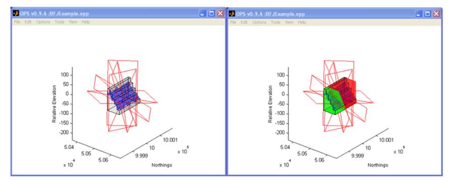
Figure 70 The water table (top) and domains (bottom) displayed in the ops
control window

Now select Options ‘
Use existing joints and leave the ‘scale factor’
and ‘spacing factor’ set to 1 and the dip and dip direction adjustments set to
0 as this will ensure the same realisation of stochastic joints is used for
this test. Ensure that ‘stochastic’ is selected as the structure type. To run
the simulation, select Tools ‘
Run simulation, leave the number of simulations set
to 1 and specify a destination directory and new project name. The simulation
will take around 1 minute depending on your computer system specifications.
Once complete, you can view the results using the facilities previously
described. If you wish to generate a series of new simulations, select Options
‘
Use existing joints to deactivate it. In this
way, a series of projects can be generated in batch mode. The results can be
viewed individually as described above or as an ensemble by using File
‘
Load ‘
Batch ‘
Block Model Analysis and selecting all the
projects you have generated.

 

5.3
Batch Processing

There are several options available to the
user who has run a series of simulations as described above and wishes to use
these as the basis for further analysis. For example, to perform an analysis of
the sensitivity of the models to joint sizes, one could use Options
‘
Use existing joints to rescale the joints by 125% and then select File
‘
Load ‘
Batch ‘
Rerun full simulations for multiple projects.
This would generate a new set of project files containing joint realisations
identical to the originals except for the increased sizes of the joints. In
fact, one could change any of the parameters in the Options menu and perform such an analysis. Note that if the only Options parameters being altered in such an analysis are those associated
with the limit equilibrium analysis (i.e. those listed under the divider bar in
the Options menu), then one can
simply use File ‘
Load ‘
Batch ‘
Rerun LE for multiple projects
which
is a much more efficient method than generating a set of new block models.

 

5.4      Sensitivity Analysis

A sensitivity analysis can be performed to
determine the significance of various assumptions such as the sizes or spacings
of discontinuities in a DFN. The analysis can be performed on one or a batch of
projects. For example, select Options ‘
Use existing joints and set the scale factor to 2, then click OK. For any projects
already containing a previously generated DFN, the software will utilise the
same DFN but increase the size of the joints by 200%. Once again, load the
sample project titled ‘BFJExample.opp‘ and then
select Tools ‘
Run simulation. Leave the number of simulations set to 1 and specify a name such as ‘BFJExampleJntsResized‘. Once the simulation is complete and
the Block Visualiser window appears, you will notice the presence of many more
unstable blocks. Bench 1 was deemed stable when the original DFN was used but
now contains several large wedges.

To
compare the simulations quantitatively, select File ‘
Load ‘
Batch ‘
Block Model Analysis and select both ‘BFJExample.opp‘ and ‘BFJExampleJntsResized‘.
The ‘Project Properties’ window appears indicating the number of blocks found
in each project. Obviously, an increase in joint sizes will normally yield more
blocks due to the increased numbers of joint intersections. Close this window,
then select Options ‘
Block Volumes from the Block Model Analysis window. The chart in the centre is of
interest here as it shows the block size distribution curves for each project.
To make the chart more readable, select Axes ‘
Log X and then click on the
middle chart. The horizontal scale will now become logarithmic allowing the two
curves to be more readily distinguished. The curve corresponding to the resized
DFN will be to the left of the other, indicating that the doubling in joint
sizes has increased the fragmentation of the rock mass.

Currently,
data for all blocks detected in the projects are being used. To limit the
analysis to unstable blocks, select Edit ‘
Filter data based on FOS and then set the upper
factor of safety limit to 1.2. Now reproduce the block volume chart as before to
see the block size distribution curves for these unstable blocks. Filters are
also provided to limit the data to a single bench or a range of block volumes.

Other
Block Model Analysis tools that are useful for such sensitivity studies include
Options ‘
Factors of Safety, Removal Forces
and Removal
Vectors.

 

6
TroubleShooting

Symptom	Possible Solutions
‘Run Simulation’ fails to produce a block model or the block model contains errors.	This can occur if the interaction between the discontinuities and the bounding volume geometries produces ‘degenerate’ geometries. Try using a simpler bounding volume (e.g. cube). Can a block model be created? If so, try tweaking your pit geometry slightly. If you are using a user defined model, reduce the number of benches. If you are using a surface model, reduce the number of facets in the surface (i.e. produce a simplified version). If not, try deactivating a discontinuity set that may be interacting ‘poorly’ with another set (e.g. combine two sets with similar orientations into one). Check that deterministic discontinuities (e.g. planes or surfaces) have not been loaded or defined multiple times. Only limited checking of this is performed and multiple definitions of the same discontinuity will cause the block modelling algorithm to fail. Try using reduced numbers/simpler representations of discontinuities.
‘Run Simulation’ takes too long to complete a block model.	Can the complexity of the pit geometry be reduced (e.g. use a user defined model rather than a triangulation, or reduce the number of benches/ size of benches)? Can the number of discontinuities be reduced (e.g. only include the discontinuities that are structurally significant for the problem being studied)? Can you specify an active depth rather than simulate the entire bounding volume? Have you specified any domains? If so, ensure you use the simplest triangulations possible as more complex domains can dramatically slow down the joint generation process.

 

7
Feedback

 

Please send feedback and bug reports to OPSFeedback@csiro.au.

 

8       References

Baecher G.B. Lanney
N.A. & Einstein H.H. (1977) ‘Statistical description of rock properties and
sampling’ in 18^th US Symp. On Rock Mech., Colorado School
of Mines, Golden CO, 5C1, pp 1-8

Chan L. & Goodman R. (1983) ‘Prediction of
support requirements for hard rock excavations using key-block theory and joint
statistics’, 24th Symposium on Rock
Mechanics, June 1983

Diederichs M.S. & Kaiser P.K. (1999)
‘Stability of large excavations in laminated hard rock masses: the voussoir analogue revisited’, Int. J. Rock Mech. Min. Sci., 36, pp. 97-117

Elmouttie M.K., Kr’henb’hl G. & Soliman A
(2016) ‘A new excavation analysis method for slope design using discrete
fracture network based polyhedral modelling’, Computers & Geotechnics, 76,
pp. 93-104

Elmouttie M.K., Poropat G.V & Kr’henb’hl,
G. (2010) ‘Polyhedral modelling of rock mass structure’, Int. J. Rock Mech. Min. Sci., 47, pp 544-552

Gibson W.H., de Bruyn
I.A. & Walker D.J.H. (2006) ‘Considerations in the optimisation of bench
face angle and berm width geometries for open pit mines’ in International Symposium on Stability of Rock
Slopes in Open Pit Mining and Civil Engineering Situations, South African
Institute of Mining and Metallurgy Symposium Series S44, pp 557-578

Goodman R.E. & Shi G. (1985) Block Theory and its Application to Rock
Engineering, Prentice-Hall, New Jersey

Hoek E. and Bray J.W. (1981). Rock Slope Engineering, Revised 3rd edition, The Institution of
Mining and Metallurgy, London.

Jing L. (2000) ‘Block system construction for
three-dimensional discrete element models of fractured rocks’, Int. J. Rock. Mech. Min Sci. v37, pp
645-659

Kalenchuk
K.S., Diederichs M.S. & McKinnon S. (2006)
‘Characterizing block geometry in jointed rockmasses‘,
Int. J. Rock Mech. Min. Sci., 43, pp
1212-1225

Lu J. (2002) ‘Systematic identification of polyhedral rock blocks with
arbitrary joints and faults’, Computers
& Geotechnics, v29, pp 49-72

Lyman G.
(2003) ‘Stereological and Other Methods Applied to Rock Joint Size Estimation ‘
Does Crofton’s Theorem Apply?’,
Mathematical Geology, Vol. 35, No. 1, pp 9-23

Mauldon
M. & Mauldon J.G. (1997) ‘Fracture sampling on a
cylinder: from scanlines to boreholes and tunnels’, Rock Mech. Rock Engng., 30(3), pp 129-144

Oddie
M.E. & Pascoe M.J. 2005. Stope performance at Olympic Dam Mine. Ninth
Underground Operators’ Conference Perth, WA, 7 – 9 March 2005

Poropat G.
& Elmouttie M. (2006)  ‘Structural
modeling of open pit mines’ in International
Symposium on Stability of Rock Slopes in Open Pit Mining and Civil Engineering
Situations, South African Institute of Mining and Metallurgy Symposium
Series S44, pp 125 ‘ 132

Ryan T.M.
& Pryor P.R. (2000) ‘Designing catch benches and interramp
slopes’ in Slope Stability in Surface
Mining, Hustrulid, McCarter & Van Zyl (Eds.),
Chapter 3, pp 27-38

Tonon F.
& Chen S. (2007) ‘Closed-form and numerical solutions for the probability
distribution function of fracture diameters’, Int. J. Rock. Mech. Min Sci. v44, pp 332-350

Vose D.
(2001) Risk Analysis ‘ A quantitative
guide. Revised 2^nd edition, John
Wiley & Sons Ltd, New York

Wang, L.G., Yamashita, S., Sugimoto, F., Pan, C., & Tan, G. (2003)
‘A Methodology for Predicting the In Situ Size and Shape Distribution of Rock
Blocks’, Rock Mech Rock Eng 36(2): 121-142

Warburton
P. (1980) ‘A stereological interpretation of joint trace data’ Int. J. Rock. Mech. Min. Sci. & Geomech. Abstr. Vol 17, pp 181-190

Warburton
P. (1981) ‘Vector stability analysis of an arbitrary polyhedral rock block with
any number of free faces’, Int. J. Rock.
Mech. Min. Sci. & Geomech. Abstr.
Vol 18, pp 415-427

Windsor
C.R. & Thompson A.G. (1996) ‘Block theory and excavation engineering’, Proc. Of NARMS 96, Montreal, V2, pp.
1753-1760

Zhang L.
& Einstein H.H. (1998) ‘Estimating the Mean Trace Length of Rock
Discontinuities’, Rock Mech. Rock Engng., 31, pp. 217-235

8.1      Copyright
And Software Notices

‘ Copyright Commonwealth Scientific and Industrial Research Organisation

(‘CSIRO’) Australia 16/07/2020

All rights are reserved and no part of this publication covered by
copyright may be reproduced or copied in any form or by any means except with
the written permission of CSIRO.

 

The Commonwealth Scientific and Research Organisation (CSIRO) makes no
representations about the content and suitability of this CSIRO software for
any purpose.

 

Specifically, CSIRO does not warrant, guarantee or make any
representations regarding the correctness, accuracy, reliability, currency, or
any other aspect regarding characteristics or use of the information presented
in this CSIRO software. The user accepts sole responsibility and risk
associated with the use and results of CSIRO software, irrespective of the
purpose to which such use or results are applied.

 

CSIRO gives no warranty, whether express or implied:

 

(i)        as to the merchantable
quality of the Software;

 

(ii)       that the Software or any
part thereof does not infringe Intellectual Property Rights of any third party
although at the Commencement Date, CSIRO is not aware of any such
infringements;

 

(iii)      that the Software will
be suitable for a particular purpose;

 

(iv)      that use of the Software will
provide any financial or monetary advantage;

 

(v)       that the Software is
error free; or

 

(vi)      that the Software will
not fail to operate or operate without error.

 

In no event shall CSIRO be liable for any special, indirect or
consequential damages or any damages whatsoever resulting from loss of use,
data or profits, whether in an action of contract, negligence or tort, rising
out of or in connection with the use or performance of CSIRO software.

 

This
software includes the Qhull algorithm:

Qhull,
Copyright (c) 1993-2001

The
National Science and Technology Research Centre for

Computation
and Visualization of Geometric Structures

(The
Geometry Centre)

University
of Minnesota

400 Lind
Hall

207 Church
Street S.E.

Minneapolis,
MN 55455 USA

email:
qhull@geom.umn.edu

This
software includes Qhull from The Geometry
Centre.  Qhull
is copyrighted as noted above.  Qhull is free software and may be obtained via anonymous
ftp from geom.umn.edu.  It may be freely
copied, modified, and redistributed under the following conditions:

1. All
copyright notices must remain intact in all files.

2. A copy
of this text file must be distributed along with any copies of Qhull that you redistribute; this includes copies that you
have modified, or copies of programs or other software products that include Qhull.

3. If you
modify Qhull, you must include a notice giving the
name of the person performing the modification, the date of   modification, and the reason for such
modification.

4. When
distributing modified versions of Qhull, or other
software products that include Qhull, you must
provide notice that the original source code may be obtained as noted above.

5. There is
no warranty or other guarantee of fitness for Qhull,
it is provided solely “as is”.
Bug reports or fixes may be sent to qhull_bug@geom.umn.edu; the authors
may or may not act on them as they desire.

 

This
software includes the FIST algorithm:

    M. Held
(2001):

    “FIST:
Fast Industrial-Strength Triangulation of Polygons”.

    Algorithmica 30(4): 563-596, 2001.

Copyright (C) Martin Held 1999-2009

C O P Y R I G H T

This code is provided at no charge to you for
purely non-profit purposes

and only for use internal to your institution. You
may use this code for

academic applications, following standard rules of
academic conduct

including crediting the author(s) and the copyright
holder in any

publication. This code is not in the public domain,
and no parts of it

may be duplicated, altered, sold, re-distributed
(in either source-code

or binary format), or used as a blueprint for
somebody else’s own

implementation without obtaining the prior written
consent of the

copyright holder. All rights reserved!

Free use of this code is restricted to purely
non-profit purposes within

academic research institutions. Absolutely all
other forms of use require

the signing of a non-disclosure agreement or of a
commercial license.

Please contact me, Martin Held
(held@cosy.sbg.ac.at), for commercial

evaluation and licensing terms.

D I S C L A I M E R

In any case, this code is provided ‘as is’, and you
use it at your own

risk. The author does not accept any
responsibility, to the extent

permitted by applicable law, for the consequences
of using it or for its

usefulness for any particular application.

Please report any bugs to held@cosy.sbg.ac.at.