Hydrodynamics
The general circulation of the Great Barrier Reef region is described by Burrage et al (1996) and summarized in Figure 1. The South Equatorial Current flows westwards through the Coral Sea as a number of narrow current jets controlled by the complex plateaux, seamounts and ridge topography of this ocean basin, with the most significant of these jets occurring immediately north and south of the Queensland Plateau. On approaching the western boundary of the Coral Sea, these multiple jets are steered by the Australian continental shelf to form the southward flowing East Australian Current (EAC) and the northward flowing Hiri Current. The Hiri Current flows along the shelf edge of the northern GBR into the Gulf of Papua where it forms a semi-closed cyclonic eddy. Both these boundary currents are known to impact low frequency currents on the GBR shelf (Brinkman et al., 2002). In the central GBR, upwelling due to fluctuations in geostrophic currents or northeast monsoon winds transports cool water along the bottom of the central GBR shelf to the seaward edge of the GBR lagoon. This cool water does not create a surface signature. However, the cool water may reach the surface via upwelling due to internal or barotropic shelf edge tides, island wakes, topographically induced eddies or bottom Ekman pumping.
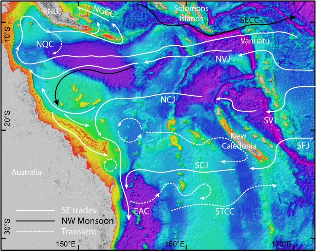
Figure 1. Bathymetry and key currents in the Great Barrier Reef region NGCC: New Guinea Coastal Current, mirroring the deeper New Guinea Coastal Undercurrent; GPC: Gulf of Papua Current, including the North Queensland Current and Hiri Gyre; SECC: South Equatorial Countercurrent; Jets of the South Equatorial Current (SEC): NVJ: North Vanuatu Jet; NCJ: North Caledonia Jet; SVJ: South Vanuatu Jet; SFJ: South Fiji Jet; SCJ: South Caledonia Jet; EAC: East Australian Current; STCC: Subtropical Countercurrent.
The southward flowing EAC is known to cause a shallowing of the thermocline along the shelf edge in the central and southern GBR, and movement of the thermocline in response to variability in the strength of the EAC is known to drive episodic upwelling and intrusions of cool water along the shelf edge of the southern and central GBR (Steinberg, 2007). Near the coast the temperature does not fluctuate in response to the tide. In shallow water near reef edges diurnal fluctuations of up to 4oC were observed by Griffin et al. (1987) and attributed to solar heating effects. Further offshore a tidal oscillation of up to 2oC was observed on a flood spring tide. Larger temperature oscillations are observed in deeper waters and are attributed to tidal pumping. The temperature lags the offshore current component by 90o (temperature minima occur at the end of the incoming tide). Griffin et al. (1987) show that a tidal current of 0.25 ms-1 may induce a vertical displacement of 60m resulting in ~1.5oC temperature variation.
The circulation and thermal characteristics of Capricorn region at the southern end of the GBR have been studied by Griffin et al. (1987). The Capricorn Channel is associated with large tides of amplitude approaching 4 m at the coast. The tide is of semidiurnal nature in the north, progressing to equal diurnal and semidiurnal behaviour in the south near Lady Elliot Is. Flood tide directions have a strong alongshore component in the GBR lagoon, becoming stronger and later further north.
The thermocline also oscillates on longer timescales (6 – 10 days) on the shelf break and slope, but this non-tidal circulation is complex and highly variable. Generally, circulation off the shelf break is dominated by pulses of north-westward flow greater than 0.3 ms-1, having a period of 6 – 10 days. This large flow is due to the cumulative effect of several baroclinic coastally trapped wave modes (Griffin and Middleton, 1986) and gives rise to a mean north to north-westward current predominantly parallel to the isobaths. The origin of these coastally trapped waves is further south beyond Fraser Island. Local wind stress contributes to circulation on the shelf, and to a lesser extent to mean flow on the shelf break. Griffin et al. (1987) postulated the presence of a large cyclonic eddy located at the southern mouth of the Capricorn Channel, generated by the EAC. This results in a north-westward backflow on the shelf-break in the vicinity of Lady Musgrove Is. The appearance and disappearance of this eddy in response to EAC fluctuations may give rise to a long period (90 day) variation in the mean current on the shelf-break.
The hydrodynamic model SHOC (Sparse Hydrodynamic Ocean Code; Herzfeld et al., 2006, https://research.csiro.au/cem/software/ems/hydro/) is employed for this study for both the regional and shelf model applications. SHOC is a general purpose model (Herzfeld, 2006) based on the manuscript of Blumberg and Herring (1987), applicable on spatial scales ranging from estuaries to regional ocean domains. It is a three-dimensional finite-difference hydrodynamic model, based on the primitive equations. Outputs from the model include three-dimensional distributions of velocity, temperature, salinity, density, passive tracers, mixing coefficients and sea-level. Inputs required by the model include forcing due to wind, atmospheric pressure gradients, surface heat and water fluxes and open-boundary conditions such as tides and low frequency ocean currents (Figure 2). The model is based on the equations of momentum, continuity and conservation of heat and salt, employing the hydrostatic and Boussinesq assumptions. The equations of motion are discredited on a finite difference stencil corresponding to the Arakawa C grid.

Figure 2. Schematic representation of major forcing inputs for the SHOC hydrodynamic model.
The model uses a curvilinear orthogonal grid in the horizontal and a choice of fixed ‘z’ coordinates or terrain-following σ coordinates in the vertical. The ‘z’ vertical system allows for wetting and drying of surface cells, useful for modelling regions such as tidal flats where large areas are periodically dry. The current implementation of the model uses z-coordinates. The bottom topography is represented using partial cells. SHOC has a free surface and uses mode splitting to separate the two dimensional (2D) mode from the three dimensional (3D) mode. This allows fast moving gravity waves to be solved independently from the slower moving internal waves allowing the 2D and 3D modes to operate on different time-steps, resulting in a considerable contribution to computational efficiency. The model uses explicit time-stepping throughout except for the vertical diffusion scheme which is implicit. A Laplacian diffusion scheme is employed in the horizontal on geopotential surfaces. Smagorinsky mixing coefficients may be utilized in the horizontal. The ocean model can invoke several turbulence closure schemes, including k-ε, k-ω, Mellor-Yamada 2.0 & 2.5 and Csanady type parameterizations. A variety of advection schemes may be used on tracers and 1st or 2nd order can be used for momentum. The model also contains a suite of open boundary conditions, including radiation, extrapolation, sponge and direct data-forcing. A generous suite of diagnostics in included in the model.
Hydrodynamic models at the 4km and 1km scale (GBR4 and GBR1 respectively) are operating routinely in near real-time within the CSIRO real-time framework (TRIKE). These model outputs are routinely posted on this website, and are publicly available via THREDDS server. The GBR4 model has been currently running routinely in near real-time since September 2010, and a hindcast archive suitable for scenario simulations exists back to that date. This period encompasses a range of forcing conditions imposed by the seasonal cycle, including extreme conditions of flood and cyclones. GBR1 began routine operation in December 2014.
The 4km model is forced with OMAPS (http://www.bom.gov.au/bluelink/products/prod_oceanmaps.html) data on the open boundaries. The tide is introduced through 22 constituents derived from the global CSR tide model. The ability of GBR4 to resolve the reef matrix is marginal; the primary role of this model is to act as a nesting vehicle between the global model and GBR1, recognising that the reef model cannot be nested directly into the global model as open boundary condition ratios should not ideally exceed 5:1. A secondary objective is the ability to directly couple to sediment transport and biogeochemistry if necessary, with acceptable runtimes, to perform longer scenario simulations. The GBR1 model is forced on the open boundaries with outputs from the 4km model (1-way nesting).
The grids to be used in eReefs are displayed in Figure 3. The GBR1 grid is extremely large, with size 510 x 2390. There are 48 vertical layers, with 1 m resolution at the surface. Although the grid is large, only 50% of the surface cells and 22% of the full 3D domain is in fact wet. The GBR4 grid is less computationally demanding; size is 220 x 500 x 44 with 1 m vertical resolution at the surface. Both models employ orthogonal curvilinear grids over the domain. These grids offer the optimum economy in terms of resolution placement, grid orientation and removal of dry cells. A higher resolution can be achieved in the areas that matter most using the minimum number of cells whose alignment is oriented parallel and normal to the dominant flow directions. Allowing the curvilinear grid to follow the coast not only naturally aligns the cells in the alongshore and cross-shelf direction (which assists stability and accuracy) but also decreases the number of land cells in the grid, leading to computational efficiencies.
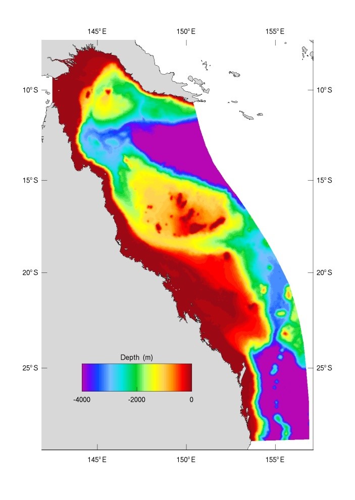
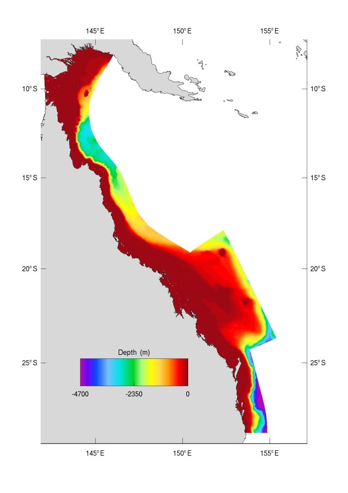 Figure 3. Model grid and bathymetry established for pilot 4km (top) and 1km (bottom) resolution model.
Bathymetry for the 1 km and 4 km models was sourced from the Digital Elevation Model of the GBR produced at 100 m spatial resolution (Beaman, 2010), https://www.deepreef.org/2010/07/06/gbr-bathy/. In the northern limits of the domain this is supplemented by the Geoscience Australia GA 2009 bathymetry (Whiteway 2009). Bathymetry from local estuaries may require supplementary data sourced from targeted field efforts.
Surface fluxes are provided by the Bureau of Meteorology’s ACCESS-R (http://www.bom.gov.au/nwp/doc/access/NWPData.shtml). This includes wind speed, rainfall, sea surface pressure, air temperature, dew-point temperature and cloud amount. These meteorological variables are used to compute momentum, heat and salt fluxes at the sea surface using bulk methods.
Both GBR1 and GBR4 include major freshwater river inputs into the lagoon. Real time flows are obtained from the Queensland Government’s river and stream monitoring network (https://www.qld.gov.au/environment/water/quality/monitoring). Twenty two rivers are presently included in the GBR1 and GBR4 models; 18 within the GBR region. The Fly River in Papua New Guinea is included due to its high discharge (consistent average over the year of 6,000 m3s-1, Harris et. al, 2004, Wolinski et. al, 2000) and high sediment loads; both natural and due to mining upstream.
Algorithms for sub grid-scale parameterisation have been developed, based on existing bottom roughness parameterisation and a unique ‘porous-plate’ approach where kinetic energy is extracted from the system by vertical mixing to account for the impact of the reef matrix on flow. This is a function of the cross sectional area the reef occupies with respect to a model grid cell. The methodology of this reef parameterisation is incorporated into the hydrodynamic models.
These models have been subject to calibration and validation, both in hindcast and near real-time, using available data, including Reef Rescue monitoring data, data from Australian Institute of Marine Science and CSIRO cruises, data from the Integrated Marine Observing System, data from Queensland Government and satellite observations. Skill assessment indicates that the models are performing well at the surface for temperature in terms of the annual and synoptic cycles. Surface salinity shows good agreement in the timing and magnitude of flow events. Biases exist in temperature and salinity at depth, which are attributed to be due to initial / boundary conditions. Diurnal and low frequency sea level correlate well with observations if a dual-relaxation open boundary scheme is used for boundary relaxation that accounts for the intrinsic temporal differences in tidal and low frequency motions.
The hydrodynamic model code has been re-configured to run in parallel on distributed memory architectures (as opposed to shared memory architectures which it can currently do). The methodology is based on master-slave data distribution, however, gather-scatter operations are performed in a slave-slave environment which introduces significant efficiencies when compared to the traditional master-slave transfers. In a benchmarking exercise, the GBR4 model was shown to outperform an identical model simulated using the MOM4 ocean code. Additionally, the GBR1 model was shown to scale linearly up to 78 processors. This allows the models to be implemented in super-computing architectures.
Two data assimilation schemes have been implemented that are suitable for use on the GBR4 grid, Ensemble Optimal Interpolation (EnOI) and Ensemble Kalman Filter (EnKF). Both schemes are able to perform state estimation, with the latter tailored to the spatial estimation of parameters (and used to estimate short wave radiation parameter distributions). There is a clear goal to try and use the DA system to reduce the error entering the model from boundary conditions and internal model parameterization. We see this as an important step forward, as sequential updating of the state in hydrodynamic models has been shown to degrade the solutions to embedded BGC models. An EnOI assimilation scheme with state update using linear adaptive relaxation has been performed to quantify its effectiveness, and demonstrate issues encountered when using such a scheme in the GBR environment.
Both the sediment transport and biogeochemistry do not operate efficiently when fully coupled to the hydrodynamic model (runtime is too slow) and must use an offline transport model as the driver. The Flux Form Semi-Lagrange Method (FFSL) used in the meteorology community has been implemented as the advection scheme in the transport model. The FFSL scheme conserves mass almost perfectly locally and can be run with longer time-steps to increase computational efficiency. The transport model was assessed against the 3D hydrodynamic model for a number of passive tracers and found to be suitable in terms of distribution of tracers, conservation characteristics and computational efficiency for driving the sediment and biogeochemistry libraries.
Development of RECOM lies at the cutting edge of modelling methodology. RECOM builds on the work performed in BLUElink, extending the capabilities of TRIKE to generate complex curvilinear grids for coastal environments and register dedicated data streams (e.g. river flow). The sediment transport and BGC, driven by the transport model, are also be included in TRIKE. The estuary models are 1-way coupled to the GBR1 or GBR4 models. A two-way coupling methodology has been developed, comprising an innovative autonomous coupling relying on push-pull data transfer rather than existing overarching orchestration methodologies such as AGRIF (Debreu et. al., 2008), but is not currently implemented.