[ Previous: Off-screen Rendering ] [ Up: Introductory Tutorials ] [ Next: Basic SQL Database ]

Introduction

In the previous tutorials, we have focused on visualising 3D mesh-based datasets in a scene. There are other types of datasets that can also benefit from the 3D visualisation capabilities of Workspace. One such type of data is volume data. There are a number of ways to think about volume data:

A stack of 2D images
A 3D image
A scalar or vector field

Workspace provides a number of datatypes and operations for working with volume data, as well as a number of widgets for visualising it. In this tutorial, we will learn about these, and understand how to use them.

In case you get stuck, a sample workflow has been provided for this tutorial.

Prerequisites

This tutorial assumes that you have completed the first two tutorials: Basic Rendering and Modifying a Model's Appearance.

Volume datasets

In the introduction, we talked a little bit about what a volume dataset is at a high level. At a lower level, volume data can be thought of as a 3 dimensional grid or matrix of data, where each cell in the matrix has a value. For example, we could have a 256x256x256 grid which contains data describing a CT-scan of a human head. Each cell in the grid would contain a value representing the density of that particular location. In a volume data set, these cells are known as "Voxels", in the same way that a cell in a 2D image is known as a "Pixel".

Let's start this tutorial by reading some volume data into the workflow:

In the Operation catalogue, find the RawVoxelReader. This operation reads raw binary data from a file without any header information. It is up to the user to know the format of their data.

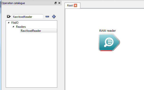
The RawVoxelReader
Note: This operation is not guaranteed to produce the same results on all platforms. It will always read the data assuming it is in little-endian format.
Click on the RawVoxelReader to select it, and in the Operation editor, enter the following properties:
- File name: Locate the file volume_sample.raw in the doc/Workspace/Examples area of the installation. This dataset is a simulation of a the spatial probability distribution of the electrons in a high potential protein molecule.
- Data size:: 8bit
- No. cells (x, y, z): 64, 64, 64
Note that the output of the operation is Array3dScalar. This represents an interface to a 3D dataset, where each cell is a scalar (floating point) value.

Visualising slices of the dataset

Now that we've an operation to give us some sample data, let's visualise some of it in the simplest way possible: as 2D slices.

From the Operation catalogue, find the GetImage3dSlice operation.

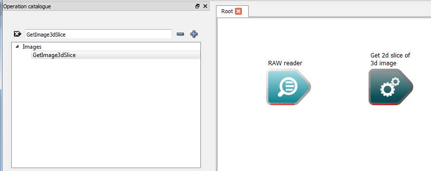
Operation to retrieve an image slice
This operation takes an Array3dScalar (similar to our scalar interface, but each cell is an RGBA value), and returns a 2D image along a user-selectable plane.
To convert our scalar data to an image, we need a Array3dScalarToImage3d operation. This will allow us to manage how our scalar data values are converted to colors.

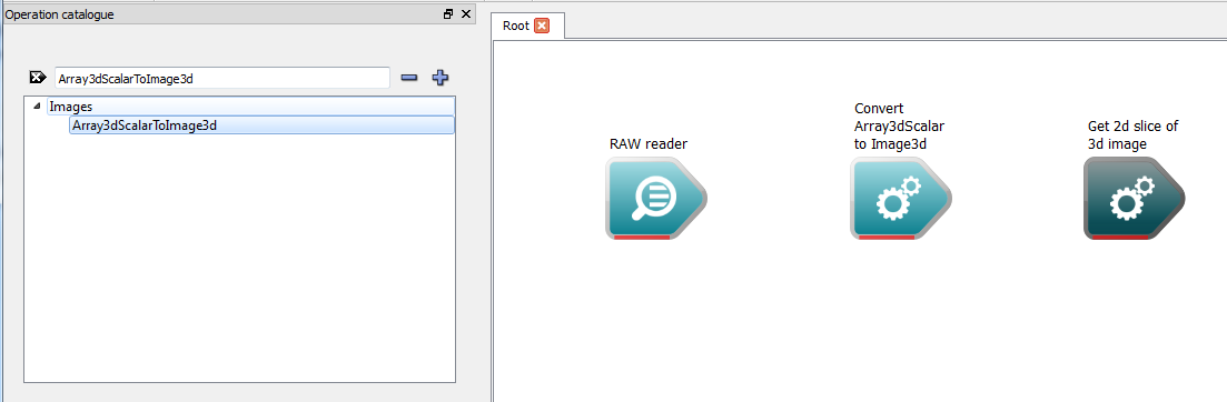
The Array3dScalarToImage3d operation
Connect the Data output of our RawVoxelReader to the Scalar matrix data input of our conversion operation.
Connect the Image output of our conversion operation to the 3d image input of our Get2dSlice operation.

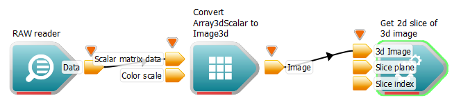
The connected operations
Create a workspace output attached to the 2d image slice output of our GetImage3dSlice operation.

If we were to execute this workflow, it would use a default color scale to convert the scalar matrix to an image. We don't want it to do this, as we want to map the colors in our scale. To do this:

From the Operation catalogue, find the ColorScaleBuilder operation and drag it onto the workspace canvas.

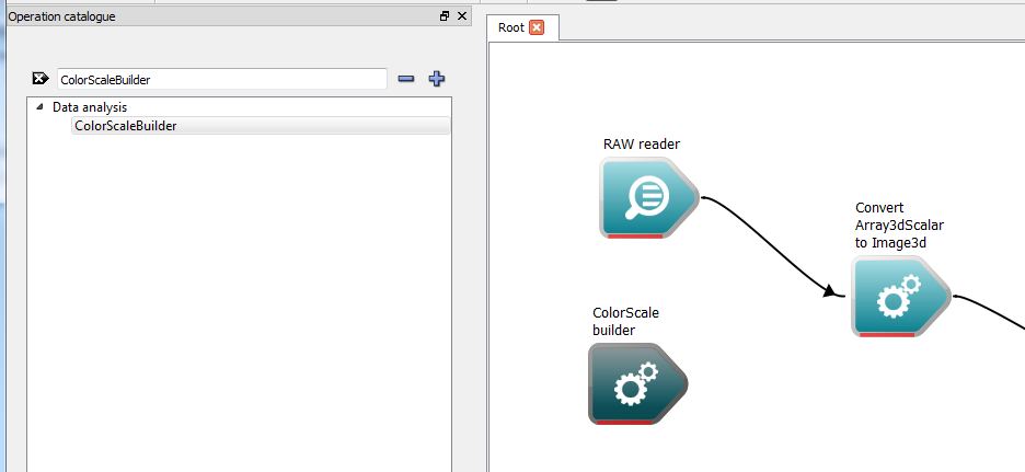
The color scale builder
Connect the Color scale output of our ColorScaleBuilder to the Color scale input of our conversion operation.
Click on the ColorScaleBuilder, and in the Operation editor, modify its inputs as follows:
- Minimum: 0
- Maximum: 255 (at 255 some of the 2D images produced from the input file will appear "blank", i.e. mostly solid blue, but as you move through the 2D images eventually you will see more meaningful images.
Create a WorkspaceOutput connected to the "Get 2d slice of 3d image" operation.
Execute the workflow

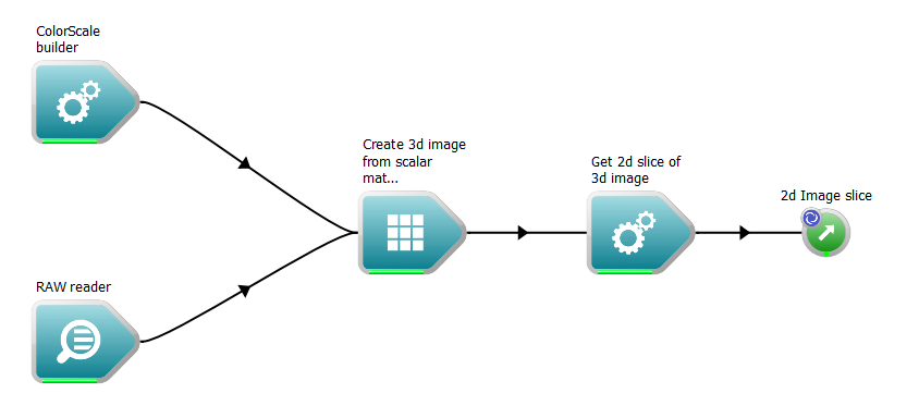
The workflow after adding the color scale builder

Right click the 2d Image slice output of the GetImaged3dSlice operation and select the "Display with ImageWidget" option. An image widget will be displayed, showing the slice.

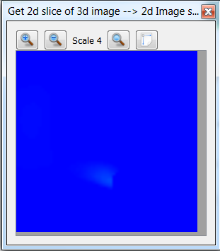
The image widget
We can use the zoom in / out buttons at the top of the widget to adjust our view of the widget.
If we click on the GetImage3dSlice operation, and in the Operation editor, modify its Slice plane or Slice index inputs, we'll see the widget update.

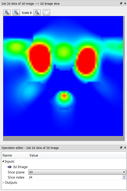
The image widget with Slice index modified

Using this technique, we can scan through the dataset by viewing each slice as a 2D image.

Visualising the dataset in a 3D scene

Now that we've seen how to view slices of a 3D dataset using Workspace, let's learn how to visualise the dataset in a 3D scene.

From the Operation catalogue, drag the CreateVolumeModelFrom3dImage operation onto the workspace canvas.

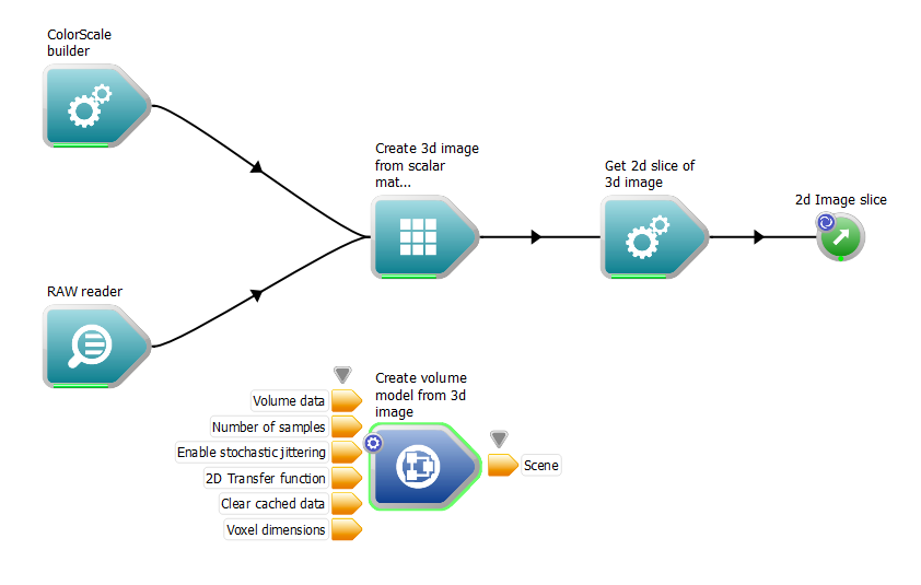
The CreateVolumeModelFrom3dImage operation
Note that this operation is actually a nested workflow - it is built up from a number of smaller operations.
Connect the Data output of our RawVoxelReader operation to the Volume data input of our new operation.
Create a WorkspaceOutput connected to the Scene output of the new operation.
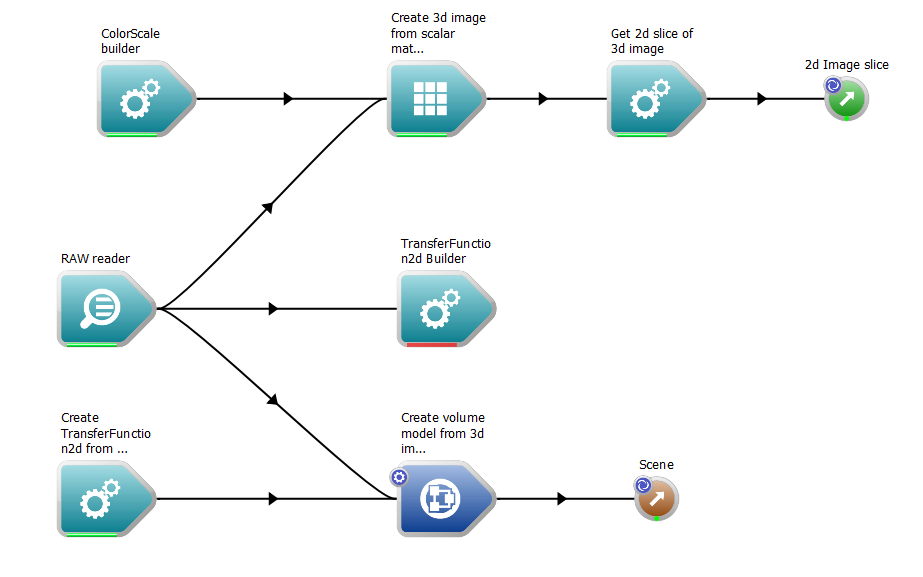
Rearrange the operations on the canvas to make a neater-looking workflow

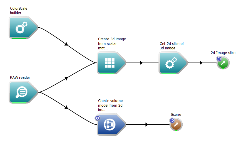
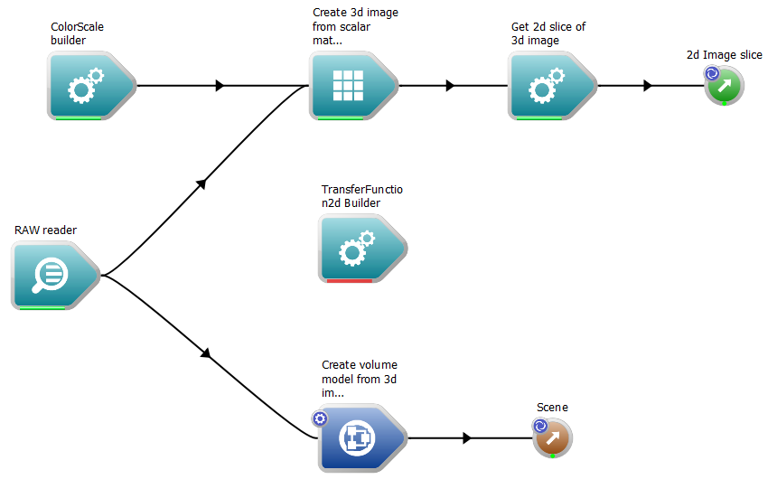
The workflow after adding the volume visualisation operations
Execute the workflow
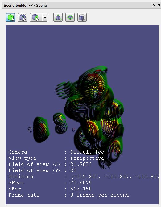
Right click on the Scene output of the new operation, and select the "Display with WSGLWidget" option from the context menu.

Initially, we will not see any data, even if we auto-fit the scene. To understand why, we need to learn a little bit about how Workspace's volume rendering technique works. The volume renderer uses a special technique known as "ray casting" in order to compute the color for each pixel in the rendered dataset. Rays are cast from the view position through the dataset, and each ray is sampled along its length in order to evaluate the final color that needs to be displayed.

If we click on our CreateVolumeModelFrom3dImage operation, we will see that it has a Number of samples input, which defaults to the value 50. In order to visualise our dataset, we will need to set this to an appropriate value. A higher value will result in a more useful image, but will result in reduced performance. A good initial value is to set this value equal to two times the maximum number of cells in our dataset (in our case, set the number of samples to 128, which is 2 * 64).

Note: depending upon the speed of your machine, and the size of the dataset being rendered, this may result in reduced performance.

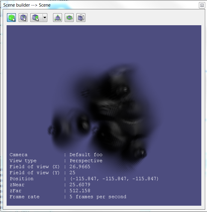
The dataset rendered in a scene with 128 samples

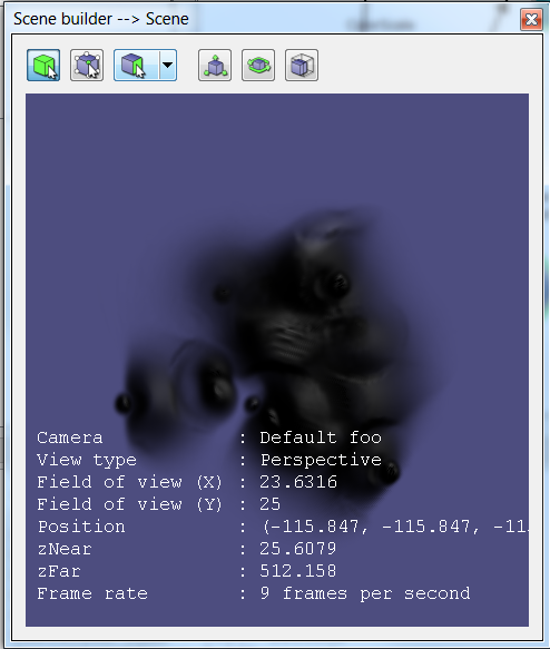
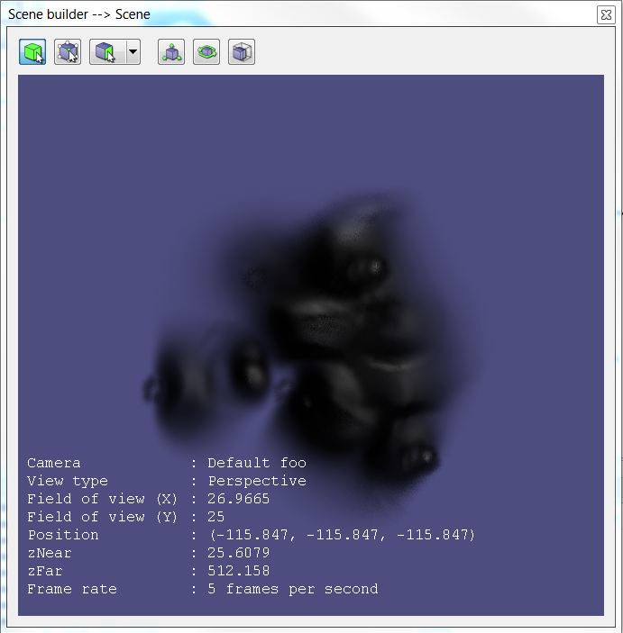
Depending upon the speed of your machine, you may find that interacting with the scene is not as fast as you would like. Reducing the number of samples will increase performance, but visual quality will be reduced. Try this now by reducing the number of samples to a smaller number (e.g. 50). Some of the visual issues that occur with low sample rates can be removed by enabling the Stochastic jittering option on the CreateVolumeModelFrom3dImage operation. This input uses a noise function to smooth out bands and rings produced by under-sampling the dataset.

50 samples, jittering on

50 samples, jittering off

So what coloring system is used? By default, the CreateVolumeModelFrom3dImage uses a grayscale transfer function, where the lowest value in the dataset is black, and the highest value in the dataset is white. In between values are interpolated linearly between the two. The transparency of pixels is computed from the 'gradient magnitude' of the dataset: areas of the dataset that are homogenous (i.e. the values around each other are the same) are transparent, and areas that are changing are opaque. This way we are able to visualise the boundaries between different 'sections' in the dataset without having the clip the volume.

Note: Clipping is possible in 3D scenes using the ClipRegion data structure, however, the ClipRegion is currently not yet supported by the VolumeShader. This feature will be added in the near future.

Transfer functions

What if we want to color specific areas of our dataset according to their data value? Workspace allows us to achieve this using what is known as a Transfer Function. Essentially, a transfer function controls the mapping of a value in the dataset to a specific color. To use a transfer function to color our dataset:

From the Operation catalogue, drag the TransferFunction2dBuilder onto the workspace canvas.

The 2d Transfer Function builder
As its name suggests, the TransferFunction2dBuilder creates a 2D transfer function The two dimensions used to compute the color of a pixel are:
- Data value: The value stored in the dataset
- Gradient magnitude: The magnitude of the rate-of-change at the particular voxel
Connect the Transfer function output of the TransferFunction2dBuilder operation to the Transfer function input of the CreateVolumeModelFrom3dImage operation.
Connect the Data output of our RawVoxelReader to the Volume data input of our TransferFunction2dBuilder. The builder will use the dataset to help us create a transfer function.
Execute the workflow.

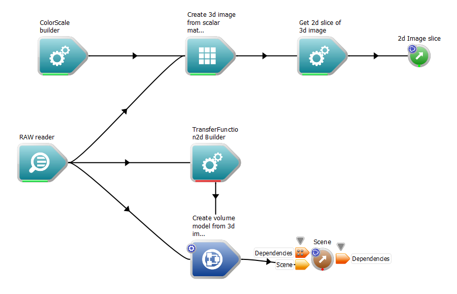
The workflow with the transfer function builder added

We will see that the volume is now invisible in our WSGLWidget. This is because we have not attempted to classify any areas of our dataset. To classify some data:

Click on the TransferFunction2dBuilder to select it. In the Operation editor, a special widget will be displayed.

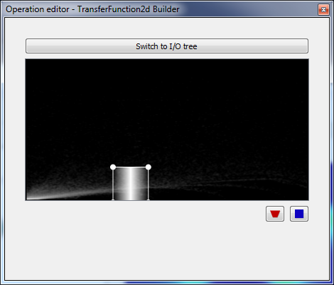
The TransferFunction2d Widget
The horizontal axis in this widget represents the data value, the vertical axis represents the gradient magnitude. We can see in the background some data has been plotted, showing us how our data is distributed in these two dimensions. Whiter areas are areas where more data is clustered.
Click the small rectangle button. This will create a rectangle widget which can be moved around by clicking and dragging.

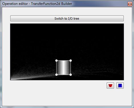
A rectangular classification area

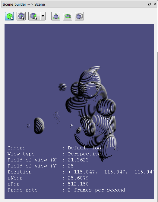
The updated WSGLWidget

Note that as the rectangle is moved, the WSGLWidget updates.
To change the color of the classification area, right click it and select "Change Color" from the context menu. A color dialog will appear where the color and opacity of the classification area can be selected. Note that the edges of the classification area fade to transparent anyway so as to allow smooth boundaries to occur in the dataset.

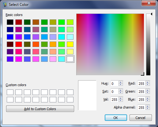
Changing the classification color

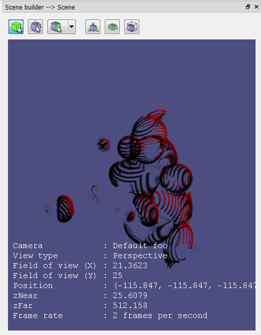
The updated WSGLWidget
Multiple classification regions can be added to the transfer function to allow different parts to be shown in relation to one another.

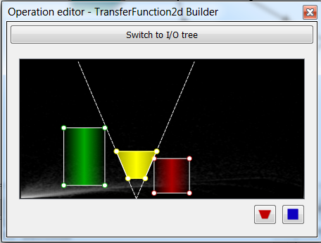
Multiple classification regions

The updated WSGLWidget, 50 samples

Using the TransferFunctionBuilder this way, we can color specific regions in our dataset according to not only their data value, but the rate-of-change of the data value. This allows us to color the boundaries between features independently.

Another technique to construct a transfer function is to use the CreateTransferFunction2dFromColorSpectrum operation. To use this operation:

From the Operation catalogue, drag a CreateTransferFunction2dFromColorSpectrum operation onto the workspace canvas.
Disconnect the TransferFunction2dBuilder from the CreateVolumeModelFrom3dImage operation.
Connect the Transfer function output of our new operation to the Transfer function input of our CreateVolumeModelFrom3dImage operation.
This operation does not need to know anything about our dataset, as its input is a simple color spectrum. Modify the color scale by clicking on it in the Operation editor.

This operation has an option to disable using the alpha as a gradient, in case there is a need to use a simple 1D transfer function (remember that transparent colors can be added to the color spectrum to allow visibility).

The workflow with the new operation added

We've now learned how to use the volume visualisation features of Workspace!

Summary

This concludes the tutorial on visualising volume datasets. You should now have an understanding of:

The datatypes used for volume rendering
How to visualize slices of the dataset
How to visualize the dataset in a 3D scene
How to apply a 2D transfer function to the dataset, and manipulate it in real-time using the transfer function editor

This concludes the set of 3D visualisation tutorials.