|
Workspace 7.1.0
|
|
Workspace 7.1.0
|
In the previous tutorial, we learned one way of visualising a MeshModel's state information using Workspace - by coloring the model's Nodes or Elements according to its state data. In this tutorial, we will learn how to visualise aspects of the model's state information using a different technique - Glyphing.
Glyphing is the process of applying "Glyphs" to each of the Nodes in a MeshModel at the time it is displayed. Depending upon the type of glypher being used, the glyphs can take many forms, and can vary in appearance from node-to-node. Some examples of glyphing applications include:
In this tutorial, you will learn:
A sample workflow has been provided for this tutorial.
This tutorial assumes that you have completed the previous two tutorials: Basic Rendering and Modifying a Model's Appearance. The steps in the tutorial build upon the workflow completed in the last tutorial - if you did not complete this tutorial, please use the sample workflow for tutorial #2 as the basis to begin this tutorial.
In this step of the tutorial, we are going to create the most commonly used type of Glypher, a SphereGlypher. The Sphere Glypher, as its name suggests, draws a Sphere at each node of the MeshModel.
Many types of MeshModels, such as 3D graph data and the outputs of particle simulations do not have Elements in them and consist only of Nodes. These MeshModels often contain state information at each node describing the particle shape. SphereGlyphers are particularly useful for providing additional depth or realism to these types of data sets.
Before we do anything else, the first thing we are going to do is change which model we're looking at, and update the selected state we are using to color its nodes. To do this:
This will update the selectable mesh reader to point to the new model, however, Workspace caches the OpenGL representation of the model, so we need to indicate to it that we want it to do away with this cached version. There are two ways to do this. The first:
Alternatively, we can:
This model contains a frame from a multi-frame particle simulation. This particular frame shows the particles after they have just collided with an object.
Now that we have a particle model, we want to create a SphereGlypher and attach it to our particle model:
Scene > Glyphers section of the Operation Catalogue, drag a SphereGlypherBuilder operation onto the workspace canvas. 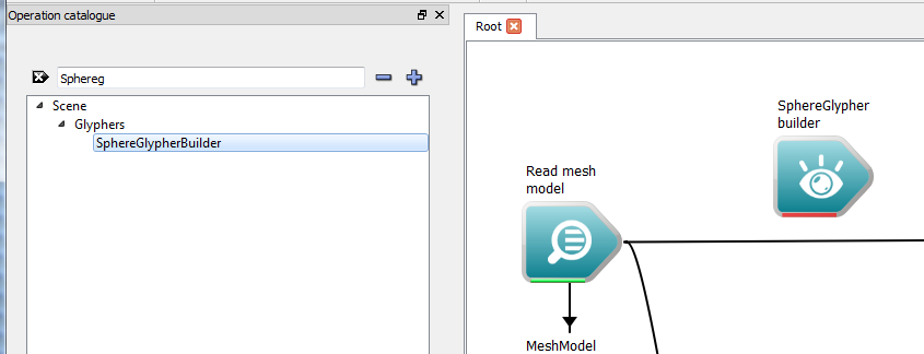
If we now Click on the SphereGlypher operation, we will see a number of properties:
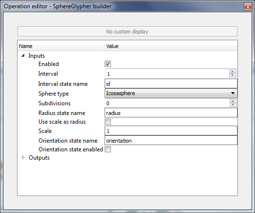
For this tutorial, we will set a few values to create an interesting visual effect:
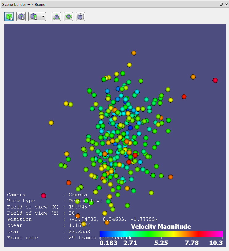
To see the results, create a WSGLWidget for our scene as we did in step 2 of the Basic Rendering tutorial. If we zoom into the model slightly, the scene should appear similar to this:
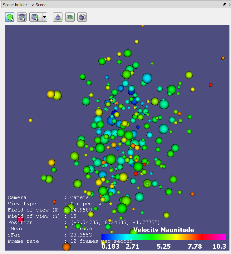
In many models, some of the states present at each node describe aspects of that node's physical appearance, such as the particle radius or orientation. The different glyphers in Workspace provide inputs which the user can use to attach states to various glyph properties.
In this part of the tutorial, we are going to demonstrate this by using the "radius" property of our model to drive the radius of our glyphs. To do this:
Often, manually entering the state name is not ideal - in many cases, it is not possible to know the names of the properties stored in the model. As we did in the previous tutorial when coloring by node-properties, we can use a "StringSelection", sourced from the list of states in the model data itself, to drive the selected property. To do this, we need another StringSelection for our "radius" property, in addition to our existing item for "velocity":
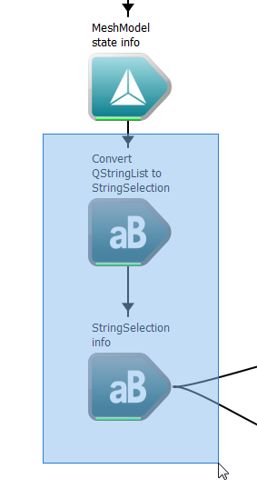
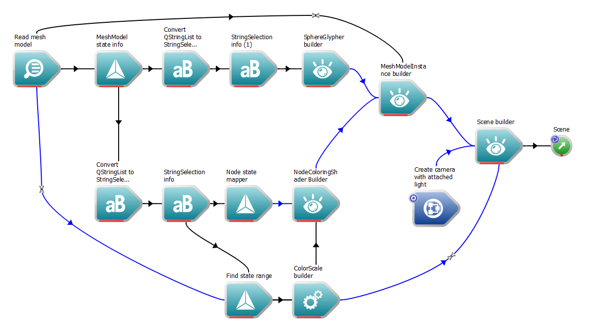
CTRL + C to copy the operations. Alternatively, click the Edit > Copy menu item in the top-left corner of the screen.CTRL + V to paste the operations onto the workspace canvas. We now have another StringSelection object which we can use to scale our glyphs independently of the model's color. (Note: at this point, you may be prompted to stop workspace execution. If this occurs, select 'OK' in the presented dialog box.)At this point, the WSGLWidget should display exactly the same view we had before - we have only changed how the radius state name is sourced. Our workflow should look similar to this:
In addition to the sphere glypher described in section 1, Workspace supplies a number of other useful glyphers. This section provides a brief overview of the different glyphers that are available out-of-the-box, and how to use them.
In some situations, instead of using perfectly spherical particles, some models use particles which are approximations of randomly shaped particles. Superquadric particles are one type of approximation. The Superquadric Glypher applies a 3D equivalent of a 'rounded rectangle' at each node in the model, where each shape can vary in its radius (independently in the x, y and z directions), its orientation, and its shape (i.e. whether it is more spherical or rectangular). All three of these properties can be set manually for all particles, or extracted from state-data.
The Vector Glypher draws vectors (arrows) at each node in the model. Unlike the other glyphers, the vector glypher uses NodeMappers to obtain the values for each of its per-node variable properties (length and direction). By default, if no direction mapper is supplied and the glypher is applied to a model containing a surface mesh, it will apply glyphs representing the surface normals at each node in the mesh.
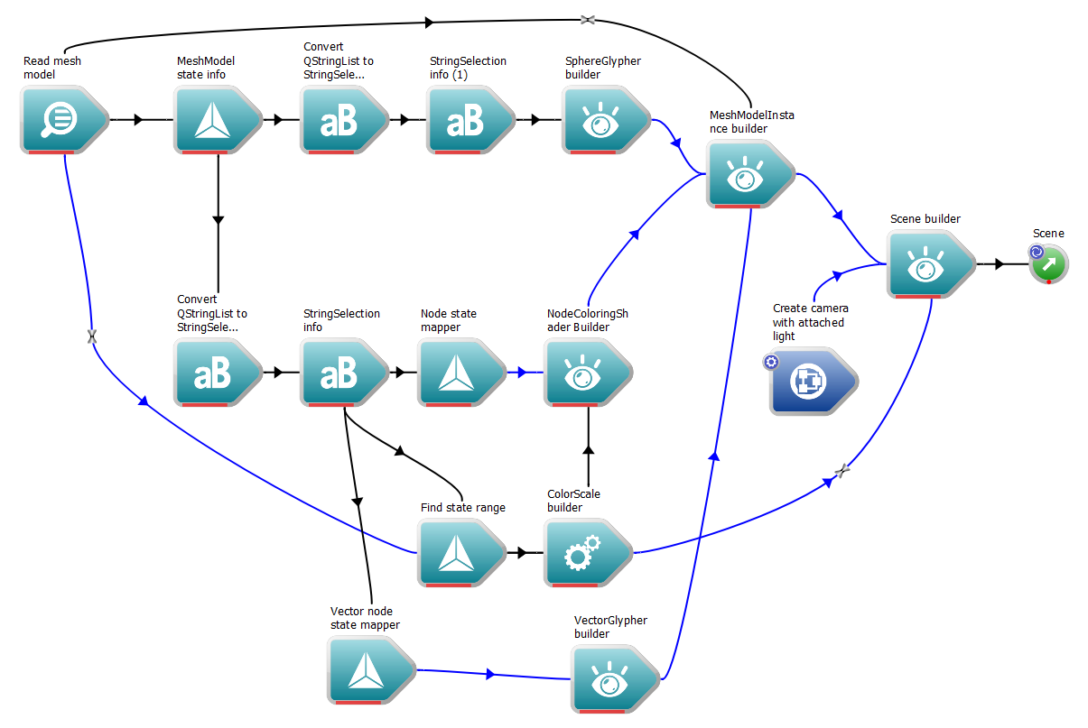
Workspace allows multiple glyphers to be applied to the same model at the same time. In our example, we are going to apply a VectorGlypher on top of our exiting SphereGlypher. To do this:
Scene > Glyphers section of the Operation Catalogue, drag a VectorGlypher onto the workspace canvas. 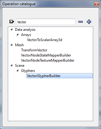
Mesh section of the Operation Catalogue, drag a VectorNodeStateMapperBuilder onto the workspace canvas. This operation differs from the NodeStateMapper, in that instead of mapping any node state (vector or scalar) to a scalar value, it maps vector node states to vector values. 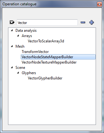
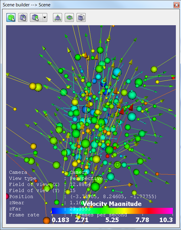
Now, if we look at the WSGLWidget, we will see that both spheres and vectors have been applied to the nodes of the model; the spheres show the size of each particle, and the vectors show its direction.
That concludes the tutorial. We have now learned:
The next few tutorials provide information about some of the other visualisation techniques: