Spark

Introduction

Spark is an open framework for simulating the spread of wildfires over terrain. The framework consists of a number of modules specifically designed for wildfire spread. These include readers and writers for geospatial data, a computational model to simulate a propagating front, a range of visualisations and tools analysing the resulting data. Spark allows the user to configure these modules in any manner. Furthermore, any number of user-defined layers can be added to the model allowing custom fire propagation models to be tested and developed. The underlying software is also designed to allow users to add custom components to the software.

This document provides an introduction to the Spark bushfire modelling components within CSIRO Workspace. Examples of how to build up full simulation work-flows are provided, as well how to visualise output and read and write data layers. Some familiarity with the basic operation of CSIRO Workspace is preferable, but not required.

Prerequisites:

Workspace installation
CSol or spark-tools plugin installation

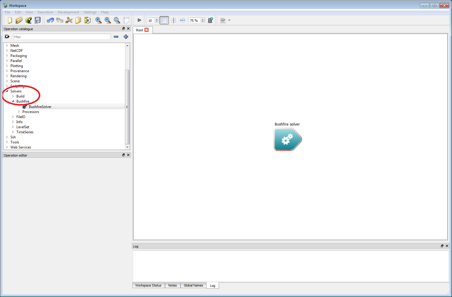
If the CSol plugin is correctly installed, a 'Solvers' item will appear in the Operation catalogue tree.

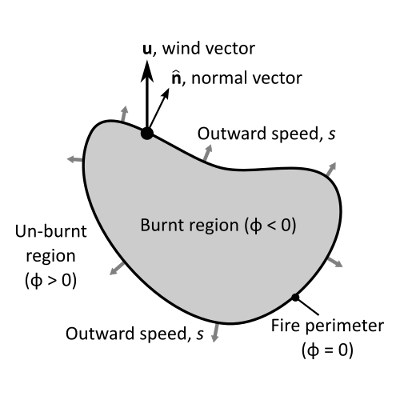
The bushfire solver uses a raster level set based method for modelling the progression of the fire perimeter. The level set has a number of advantages over other perimeter propagation models. This includes the ability to handle the merging (or breaking) of any number of perimeters, for example, allowing the full dynamics of spot fires to be modelled. The level set method works by tracking the distance to the nearest perimeter in each raster cell, φ, rather than modelling the perimeter itself. The fire perimeter is assumed to divide regions which are burnt and regions that are un-burnt. The perimeter itself is reconstructed from where φ is zero. Another advantage of the level set method is the ability to control the outward speed s at each point on the perimeter. The outward speed of a fire perimeter depends on many factors such as the local fuel type, wind conditions and topography. Rather than defining a limited number of pre-set fire models, Spark allows the user to program in any outward rate of spread for a practically unlimited number of fuel types.

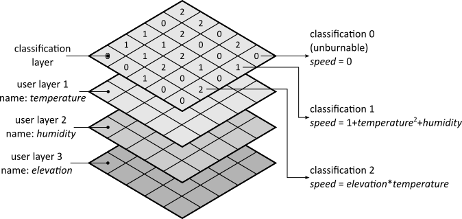
The two-dimensional level set method

The fuel types are stored in an internally defined classification layer. Zero in the classification layer is reserved for un-burnable terrain. Non-zero values each correspond to a specific fuel type, each with their own rate-of-spread function and ignition characteristics. For example, fuel type 1 could be grassland, with an associated grassland rate of spread function and fuel type 2 could be forest, with a different rate of spread function. The rate of spread models used are saved with the project, allowing detailed auditing of the model used for a particular simulation, if required. Furthermore, the framework can be used to develop and test new models which can be deployed immediately for operations or planning.

Internal raster layers

The model also requires no geospatial bounds to be specified as it uses a tile-based method. As the fire reaches the edge of a tile, a new raster neighbouring tile is created. Similarly when the fire leaves a tile, the tile is switched off to save computational resources. A set of tiles makes up a two-dimensional raster layer called a Grid. A Grid is the base structure for all CSol computations, and can be one, two or three dimensional. For most of the applications covered here, however, a two-dimensional Grid and a raster layer can be thought of interchangeably.

The implementation also supports sub-solvers, called processors. These are independent computational solvers that are run each time step. Any number of these sub-solvers can be plugged into the bushfire solver. Currently these include:

A wind-field generator from a time-series.
A wind-field generator from a gridded wind field.
A model for fire crossing of a given network, such as roads or power lines (demonstration).
A spotting model (demonstration).

Note: OpenCL drivers are required to run the Spark solver. For systems with no GPU, free drivers are available for all systems from AMD and Intel-only devices from Intel. NVidia and AMD freely provide OpenCL drivers for their GPU devices. Use of GPU drivers is recommended as this will greatly increase the speed of simulations.

Basic bushfire work-flow

Example files.

For a first example, we will build up a very basic bushfire work-flow. The final result won't look much like a bushfire (this will be improved in the next example) but it will give a good overview of how the system works. This example should also give a broad feel for the flexibility of the system, which will be built on in later examples.

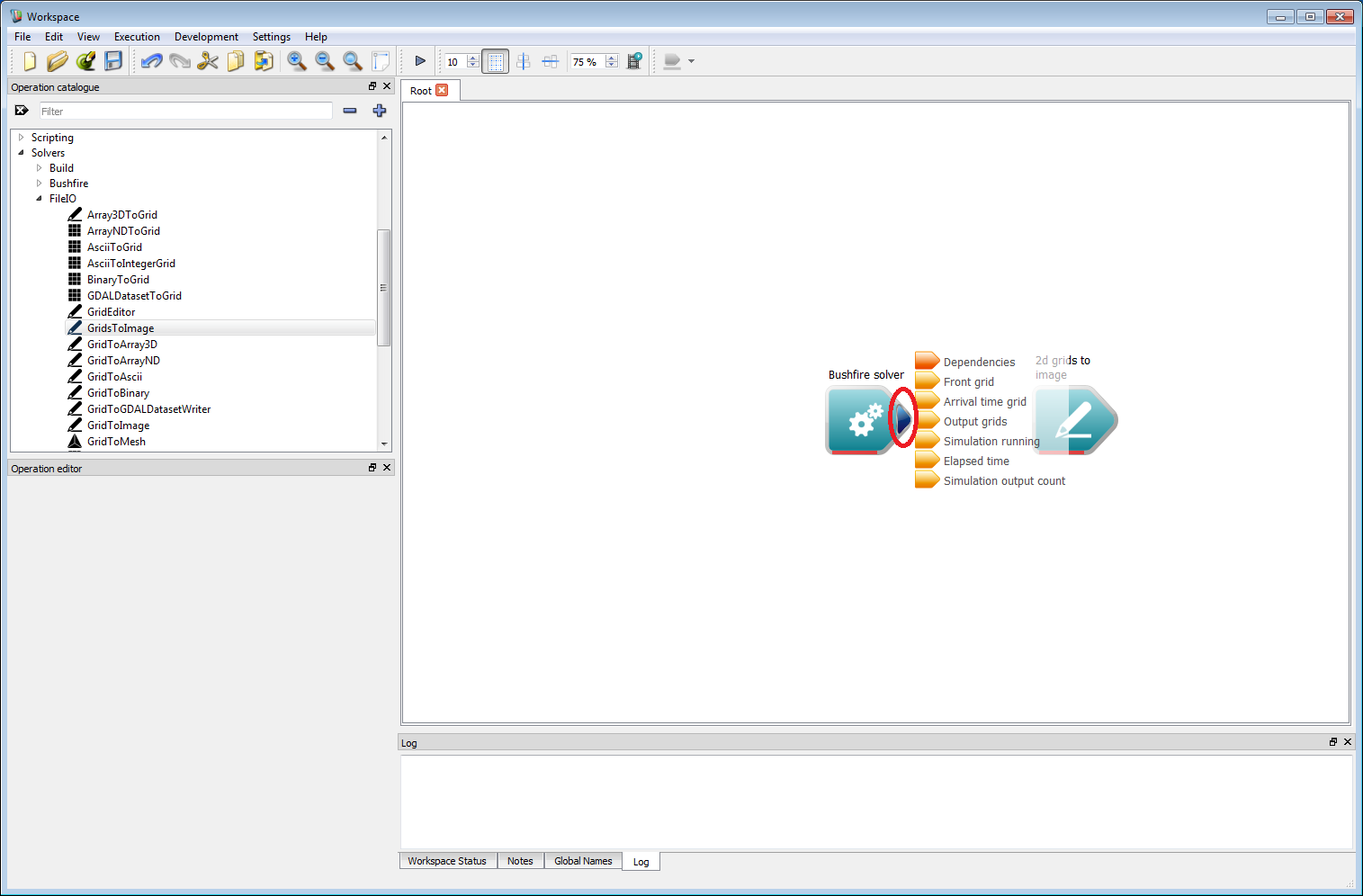
To start, we need a bushfire solver. Run Workspace and check that the Solvers item appears in the operation catalogue tree on the left hand side (circled red in the figure below). Expand Solvers and Bushfire. The BushfireSolver operation will be visible in the BF list. Left-click down on the BushfireSolver item and, holding the mouse button down, drag the item onto the white canvas on the right-hand side. The Bushfire solver operation will appear in the region as a triangular block, as shown below. Each triangular block in the white canvas region represents an individual work-flow operation, and this block represents the core operation which will carry out the computations for the bushfire simulation.

Note
All operations contain functional information in the form of a tool-tip which appears when the mouse hovers over an operation.

Basic work-flow step 1
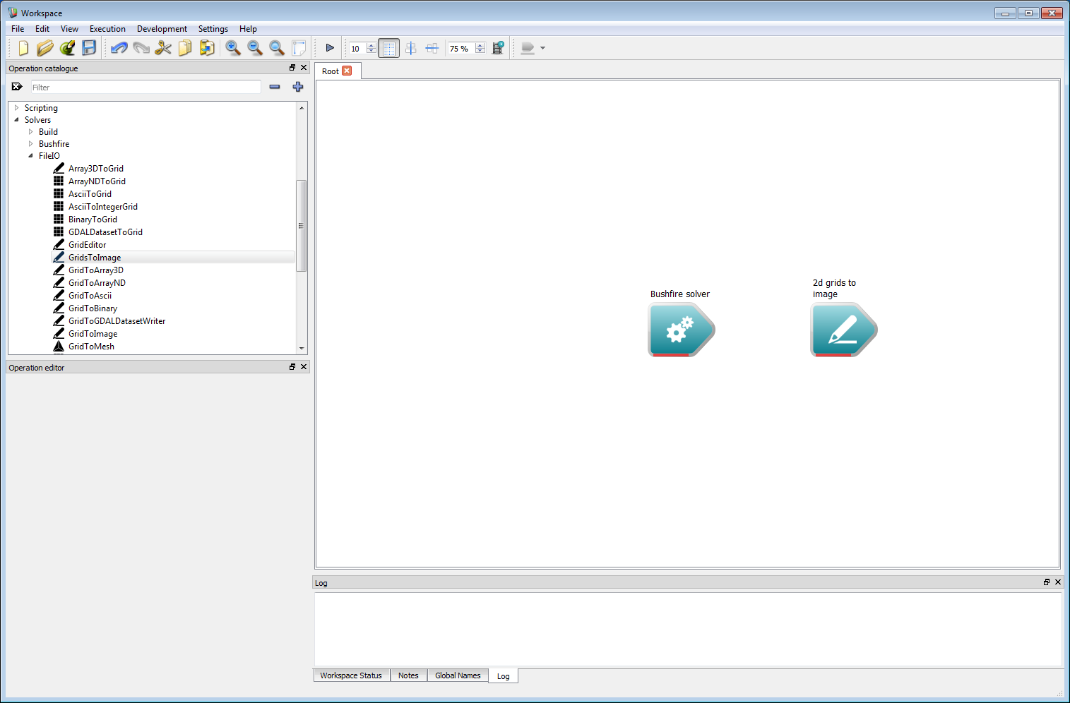
Next, we need some output. In this example it will simply be an image of the arrival time of the fire front. Other output formats exist, such as raster and vector layers, which will be covered in the following examples. For now, we will keep things simple for clarity. Input and output operations are under Solvers/FileIO on the operation catalogue tree. Navigate to FileIO and select GridsToImage. Drag this operation onto the canvas. This operation can be located anywhere, we have placed it on the right-hand side of the solver operation so the work-flow follows a left-to-right path. This operation converts a collection of two-dimensional output layers to an image which can be viewed or saved.

Warning
Ensure GridsToImage (grids plural) is selected and not GridToImage.

Basic work-flow step 2
The solver output now needs to be connected to the image input. Move the mouse over the right-hand tip of the operation block (circled red below) and a set of outputs will appear (shown as a vertical set of smaller triangular elements). Each output has an associated line of text describing the output. For this example we only require the Arrival time grid, which is a two-dimensional raster layer containing the time the fire front arrives within each raster cell. Move the mouse over this item and the output will turn green. Next, left-click on the output and, holding down the left button, drag the mouse over to the 2d grids to image operation. There will be an input element on the 2d grids to image operation called Grid data. While holding the left-hand button move over this input element and it will turn green, indicating the Arrival time grid output can be connected to the Grid data input. Release the mouse button to make this connection and a solid line with an arrow will appear joining the two operations. This joining operation is central to building work-flows in Workspace.

Note
When an operation output is selected only available operation inputs appear in the Workflow canvas, making it easy to see all the possible connections.

Basic work-flow step 3
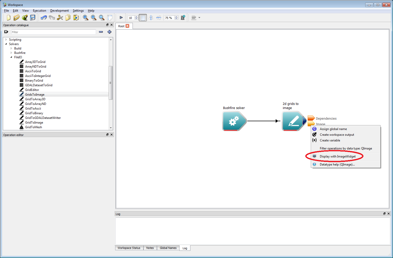
It is important to set your pixel resolution input within the 2d grids to image operation, in this case it should be set to 1 m. To view the output image right-click on the Image output of the 2d grids to image operation. Select the Display with ImageWidget (circled in red below) open from the menu that appears. An image view Widget will appear, which will initially show only a dark grey canvas. If this appears as a floating window, it can be docked with the main Workspace window using CTRL+D.

Basic work-flow step 4
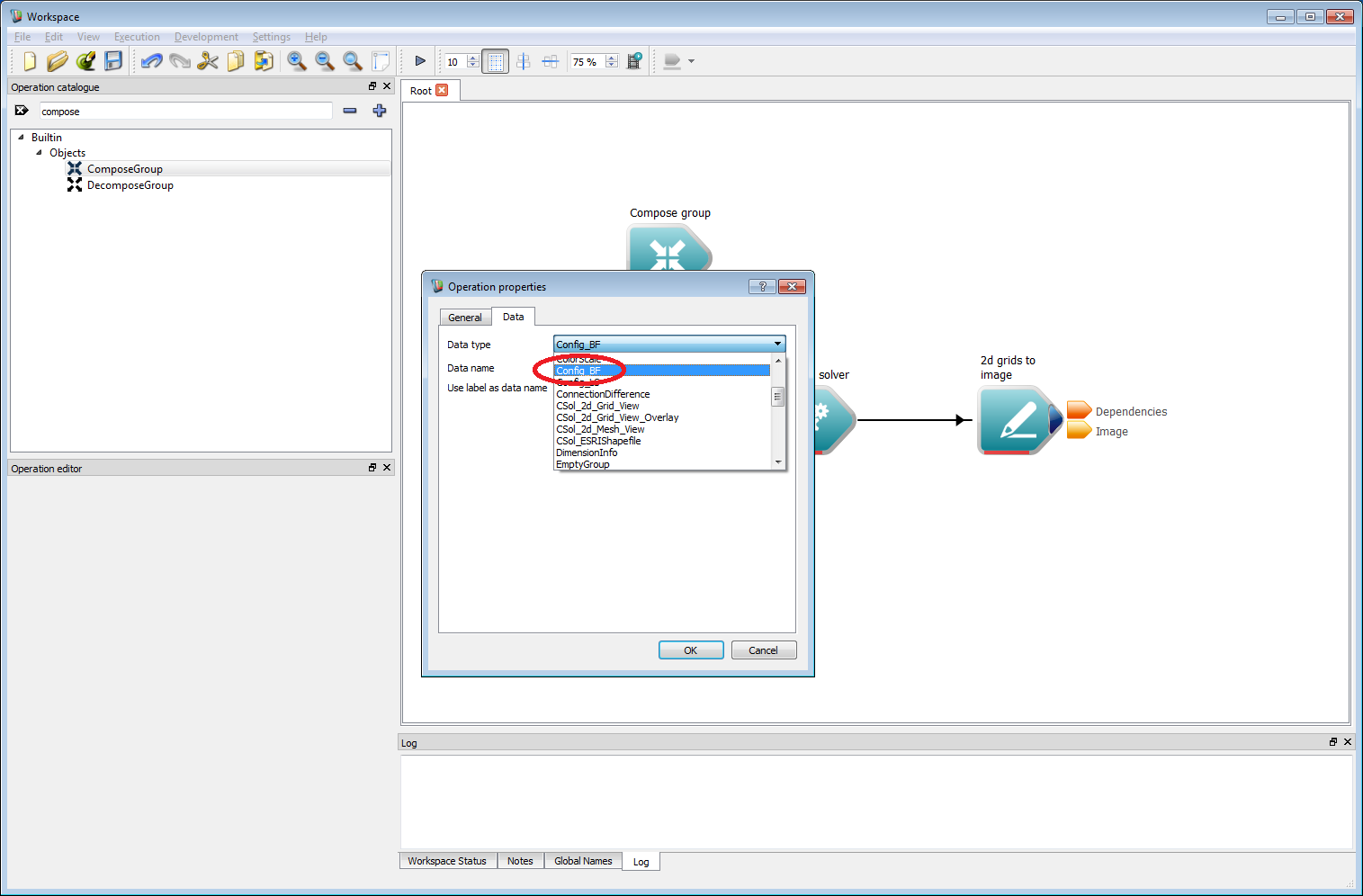
Now we have a basic output, we need to specify the inputs to the bushfire solver. There are a minimum of three required inputs for the bushfire solver: a set of configuration parameters, at least one rate of spread model and a starting point or raster starting layer. The first of these is a set of solver-specific configuration parameters. Parameter sets in the Workspace environment are called Groups, and are created using an operation called Compose Group. Rather than looking through the operation catalogue tree for this, the name can be entered into the search box at the top of the catalogue (circled red). Drag the Compose Group onto the canvas and an Operation Properties dialog box will immediately appear. This box allows the type of group to be set. Here, we need a bushfire configuration data type called Config_BF. Press OK once this has been selected.

Basic work-flow step 5
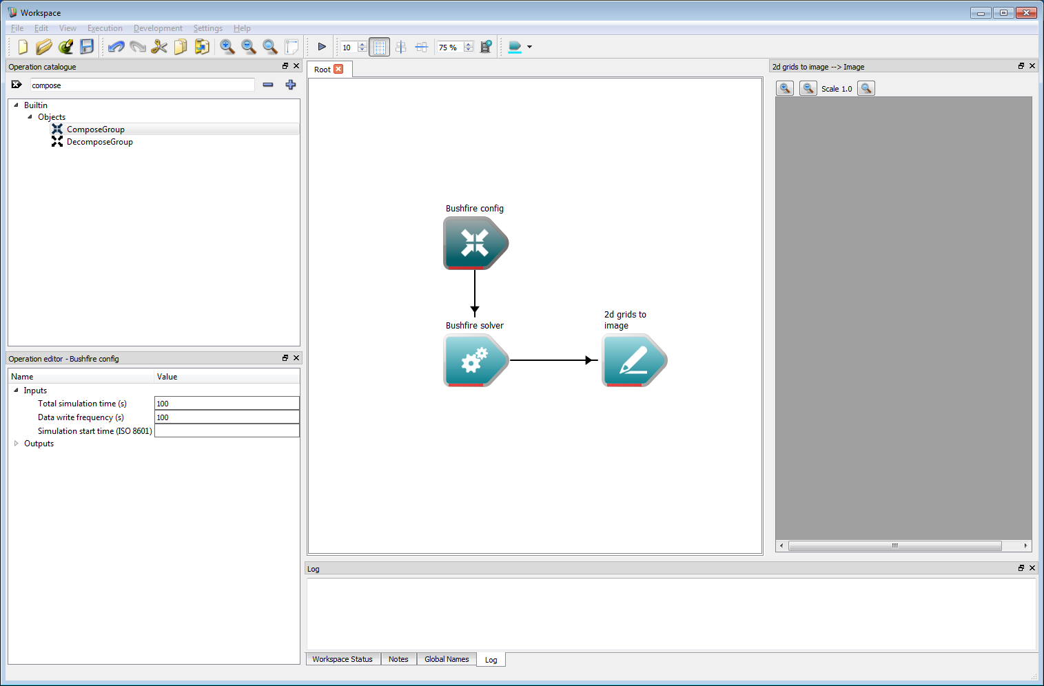
The Object group output from the Compose Group operation can now be connected to the Configuration input on the bushfire solver. Left-clicking on the Compose Group operation (re-labelled Bushfire config in the figure below by double clicking on the operation and changing the label) opens the operation inputs in the operation editor panel on the bottom left of Workspace. Editable inputs for the configuration include:
- The total simulation time in seconds.
- The data write frequency or the period between data output from the solver, in seconds.
- The simulation start time, which is a date stamp used to set the start of the simulation. All time-based user inputs, for example time-stamped NetCDF data files and time series inputs, are sampled relative to this time.
Note
The start time uses the ISO 8601 date format, for example 2010-01-01T13:00:00+10:00, for 1st January 2010, 1pm in Sydney time (UTC+10), or 2010-01-01T13:00:00Z, for 1st January 2010, 1pm in UTC time. If the start time is left blank, the simulation start time is set to a default of epoch time zero (midnight 1st January 1970).

Warning
If the start time does not specify a UTC time zone the local system time will be used. To ensure portability of workflows the UTC time zone should be specified.

For now, the total simulation time and write frequency should be set to 100 seconds.

Note
Operations can have any labels. These can be edited by double-clicking on the operation and editing the Label. The Compose Group label in this example has been changed from the default 'Compose Group' to 'Bushfire config' for clarity.

Basic work-flow step 6
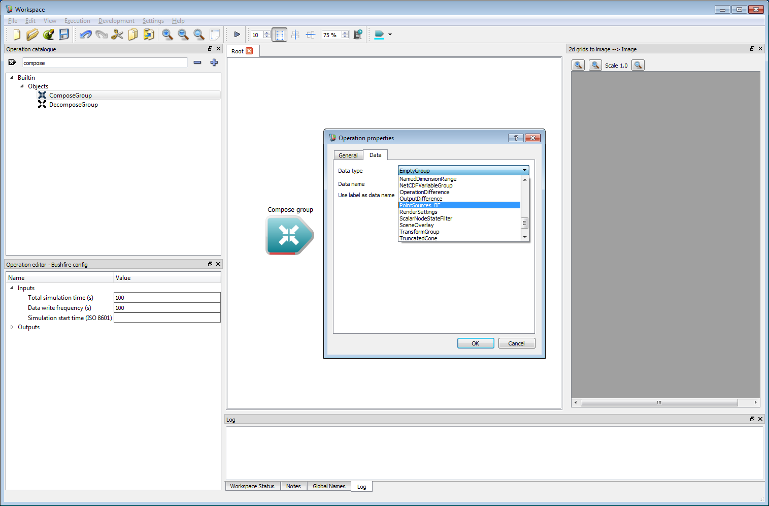
Now that the configuration options are set, some starting locations of the fire are needed. There are two ways to specify starting conditions, either a raster layer or circular point sources. Circular point sources are used in this example as they can be programmed. Again, a Group is used for specifying the point sources, requiring a Compose Group operation. Create a new Compose Group operation and select PointSources_BF from the drop-down list.

Basic work-flow step 7
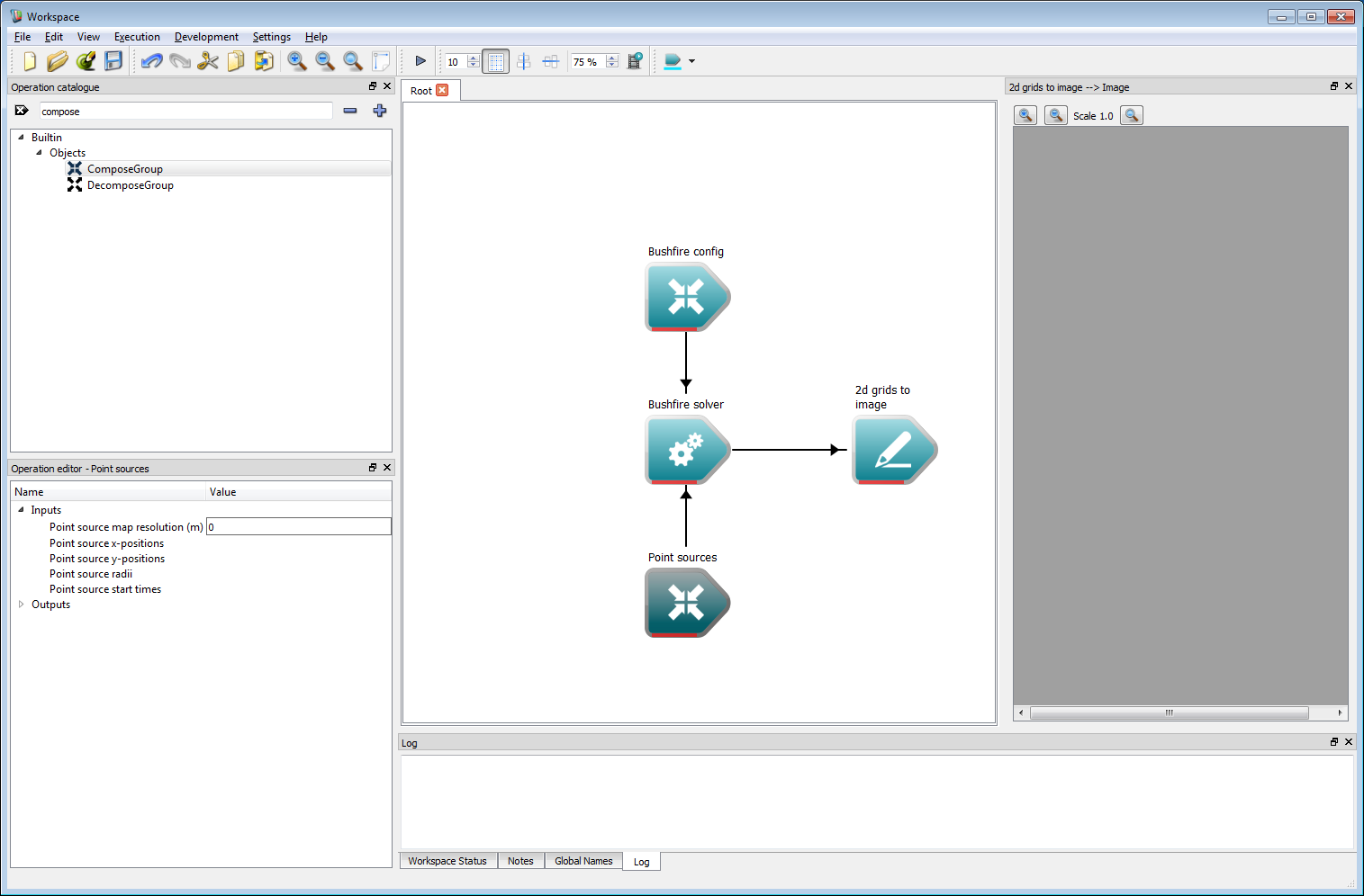
The Compose Group has been re-labelled Point Sources and moved below the solver to save space. Connect the Object group output from Point Sources to the Initial point sources input on the bushfire solver. Clicking on the Point Sources operation shows that the inputs to the operation can't simply be entered in the operation editor. These are lists of points, positions, radii and start times which need to be specified using a different method.

Basic work-flow step 8
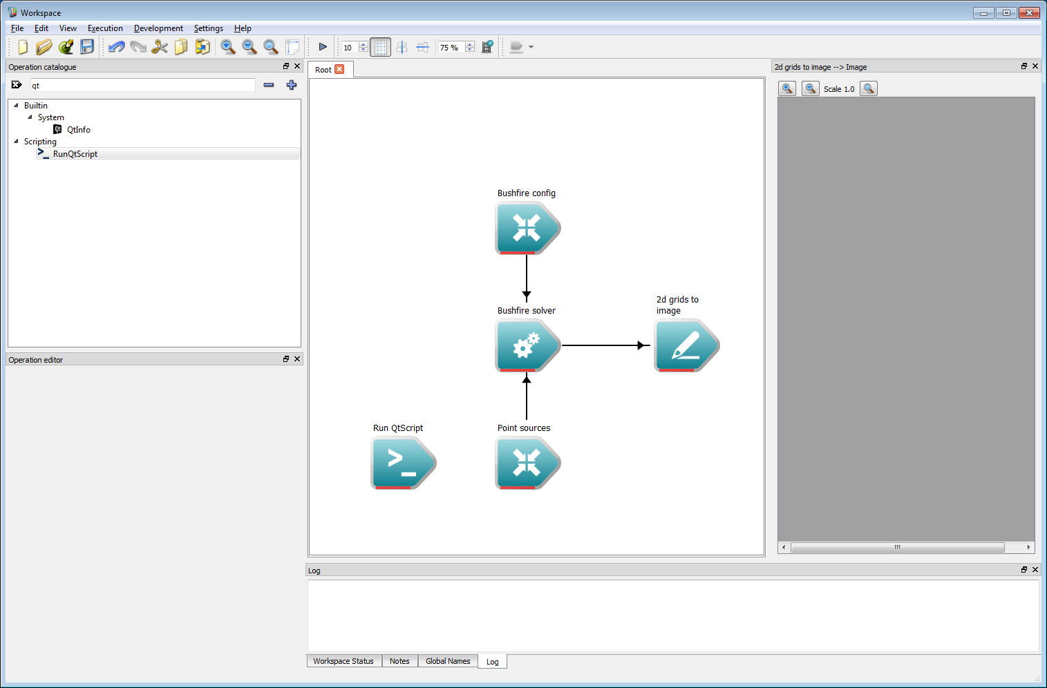
There are a number of ways of specifying lists within the Workspace environment. As a demonstration we use a simple Qt script in this example. Scripts are slightly more involved than other types of operation but allow great flexibility in work-flow operation. To implement a script, first add a Run QtScript operation to the work-flow.

Note
Qt script uses the ECMAScript, or JavaScript, standard and allows the full range of functionality of this language. Alternatively, a Python script operation also exists and is compatible with this example, if preferred.

Basic work-flow step 9
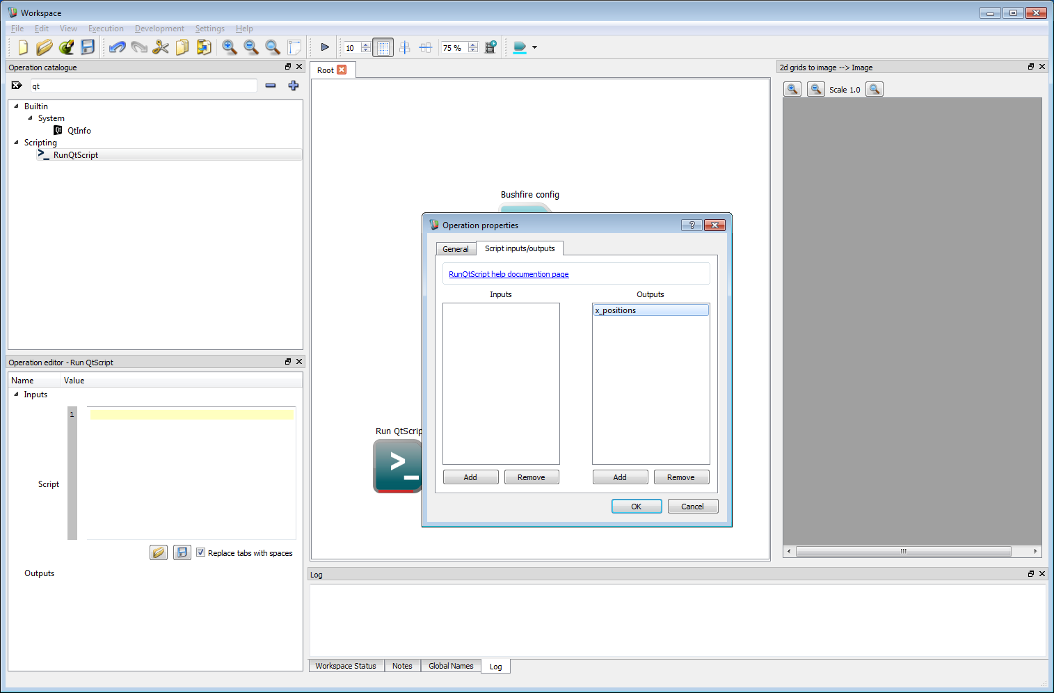
Next, double click on the Run QtScript operation to bring up the Operation properties dialog box. Select the Script inputs/outputs tab. Unlike other operations, script operations allow the user to define which inputs and outputs are used in the operation. We require three lists to specify each point source, a list for the point source x-position, a list for the y-position and a list for the radius of each point source. An optional fourth list of times at which the fires ignite can be used, otherwise all of the fires are assumed to start at the start of the simulation. Each of these can be added as outputs by clicking on the Add button under the output column. This will create an output called newOutput. Double clicking on the newOutput entry allows it to be renamed.

Basic work-flow step 10
Create three named outputs called x_positions, y_positions and radii. No inputs are required for this example but can, of course, be used for more complex work-flows. Click OK to close the properties dialog box.

Basic work-flow step 11
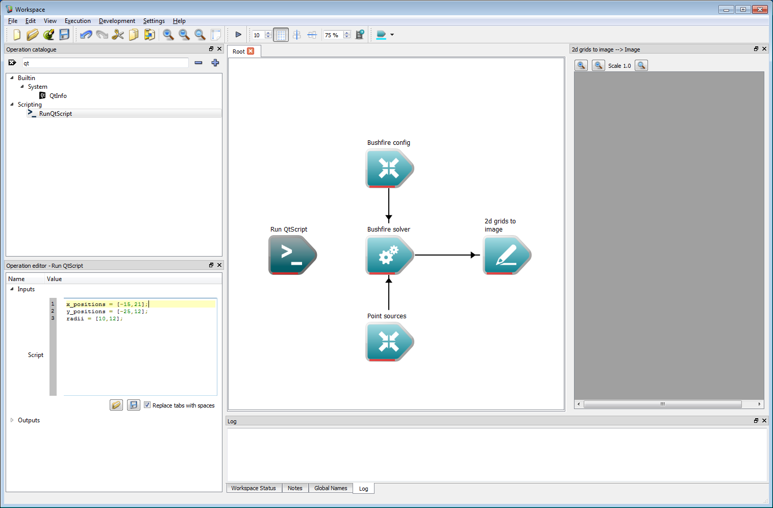
The script input will appear in the operation editor panel. The starting positions are specified as lists in the scripting language. For Qt Script or Python these are specified as:

x_positions = [-15,21];
y_positions = [-25,12];
radii = [10,12];

This will create two initial sources, one at an arbitrary (easting, northing) location of (-15, -25) with a radius of 10 m and a second at (21, 12) with a radius of 12 m.

Basic work-flow step 12

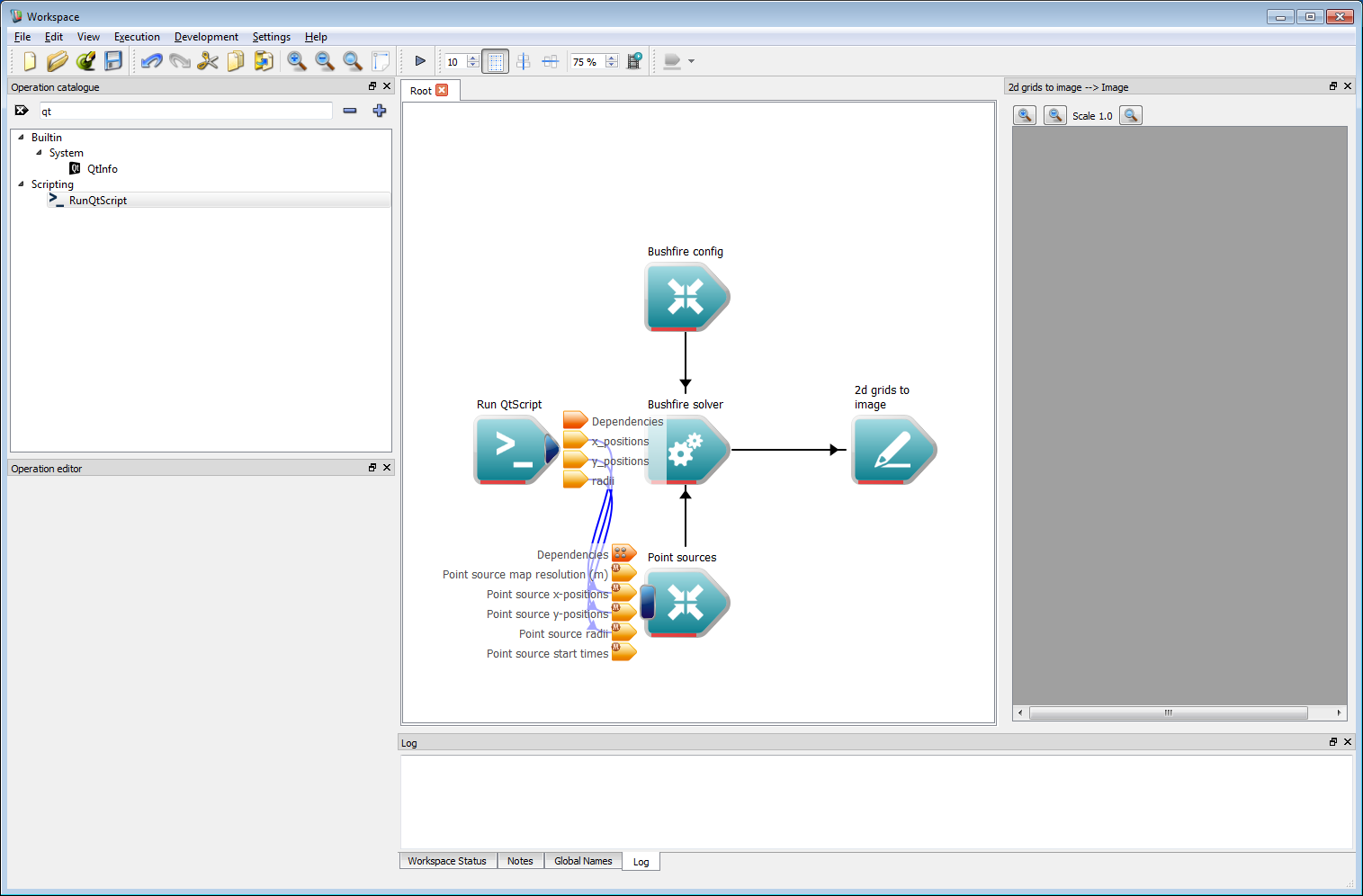
The three outputs from the Run QtScript operation need to be connected to the respective inputs of the Point Sources operation.

Basic work-flow step 13
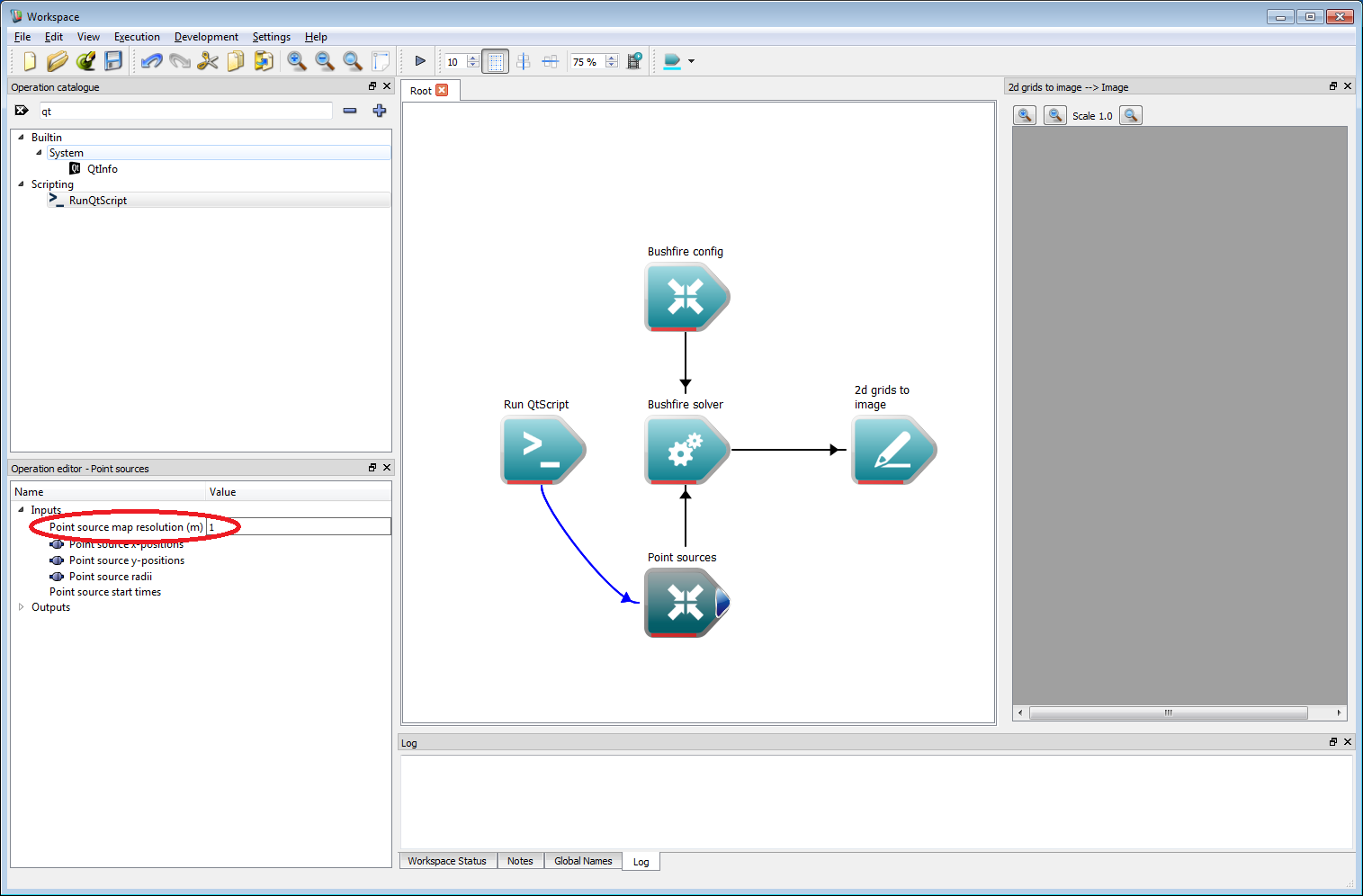
The resolution to use for the point sources must be specified. This should be set to 1 m in the resolution input of the Point Sources operation.

Basic work-flow step 14
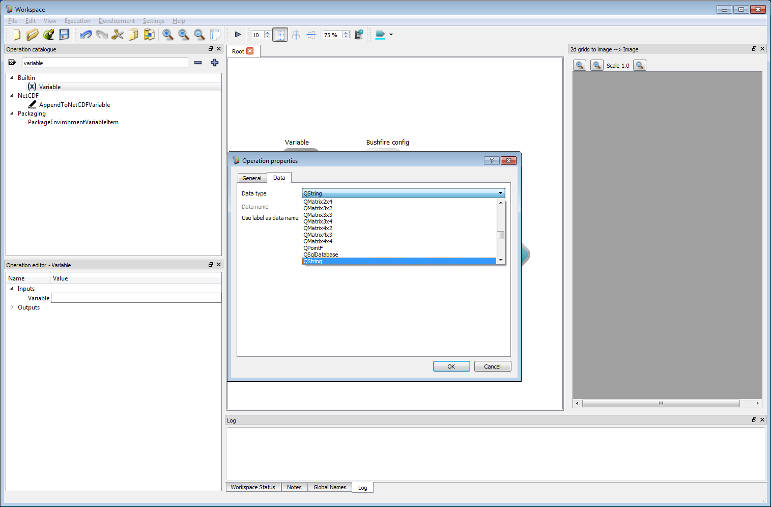
The final step is the most important. The speed function governing the rate of spread must be given to the bushfire solver. The speed function is programmable and can read from any input layer allowing complex fire behaviour models to be implemented. Here, we will simply set the speed to a constant value. The speed function is input as a text string. Here, we use a Workspace Variable operation to store and use the text string. Creating a Variable operation immediately opens the operation properties dialog box. Select QString from the data type list.

Basic work-flow step 15
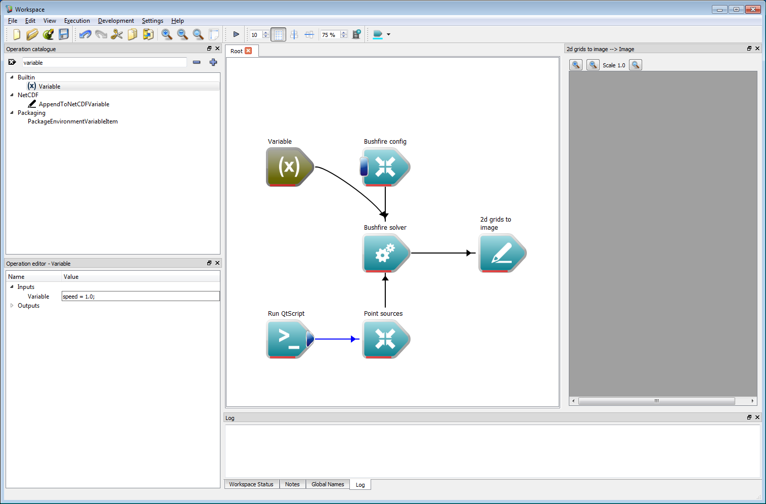
Next connect the Variable output from the operation to the Rate of spread models input on the Bushfire solver operation.

Note
There are four small dots of the Rate of spread models input, indicating that this input can take multiple values of the same type. For this input, the first string connection is used to define the speed function for classification 1, the second string input is used to define the speed function for classification 2, and so on.

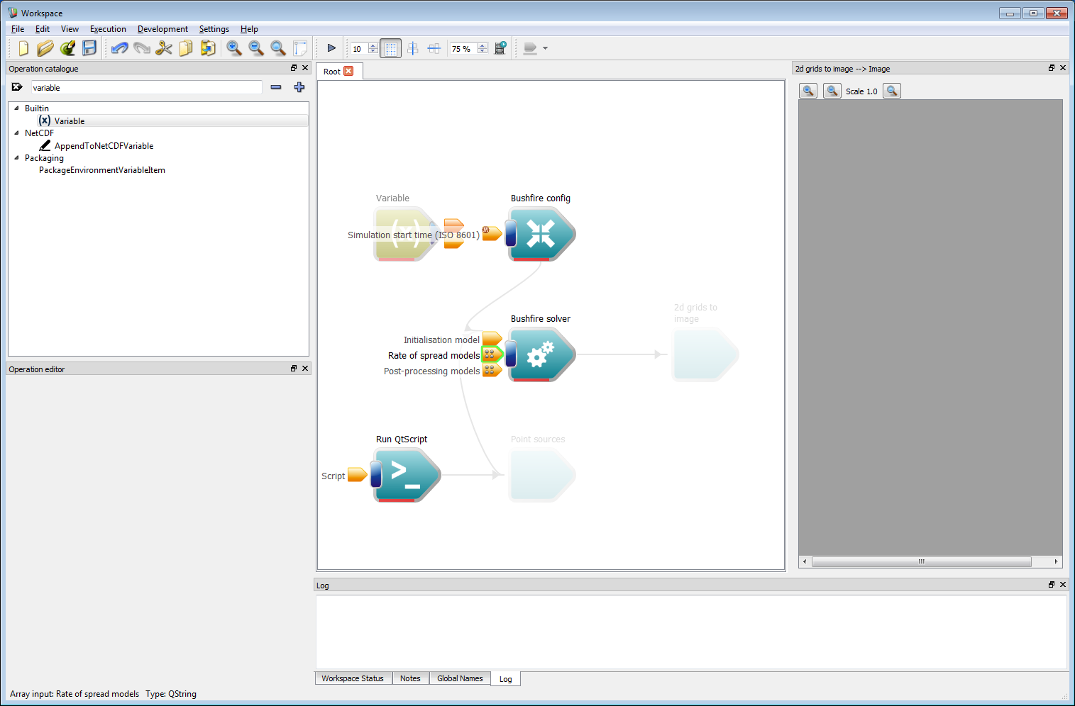Basic work-flow step 16
Left click on the Variable operation to show the editable inputs within the operation editor panel. The outward speed of the front is set to a constant value of 1 m/s using:

speed = 1.0;

Warning: The speed function is compiled in C, so a semicolon is required to end statements.

Basic work-flow step 17

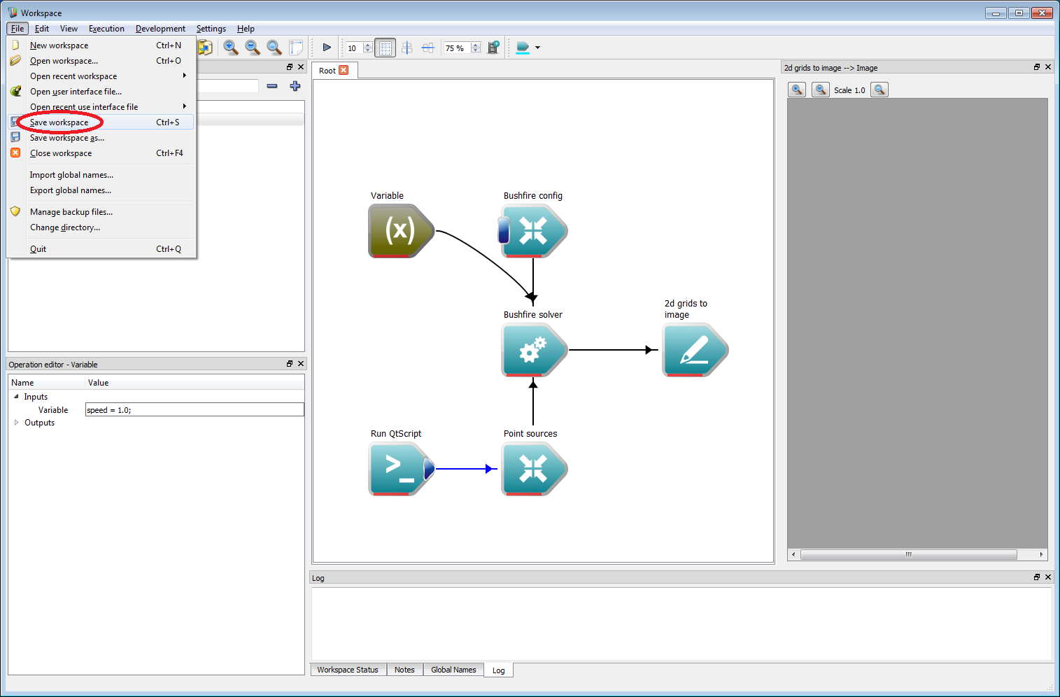
Before running a model is always a good time to save the project. To do this, go to File/Save workspace (circled in red) and save the project in a suitable location.

Note
Projects are saved with a wsx extension by default. However, this is just xml. The xml file can be directly edited or even generated by a different application, if required.

Basic work-flow step 18
Finally, press the Toggle execution button on the Workspace editor (circled in red in the image below). The simulation will start and the resulting output should be the same as the figure below. Information on the simulation is given in the log panel at the bottom. The simulation should only take a few moments to complete.

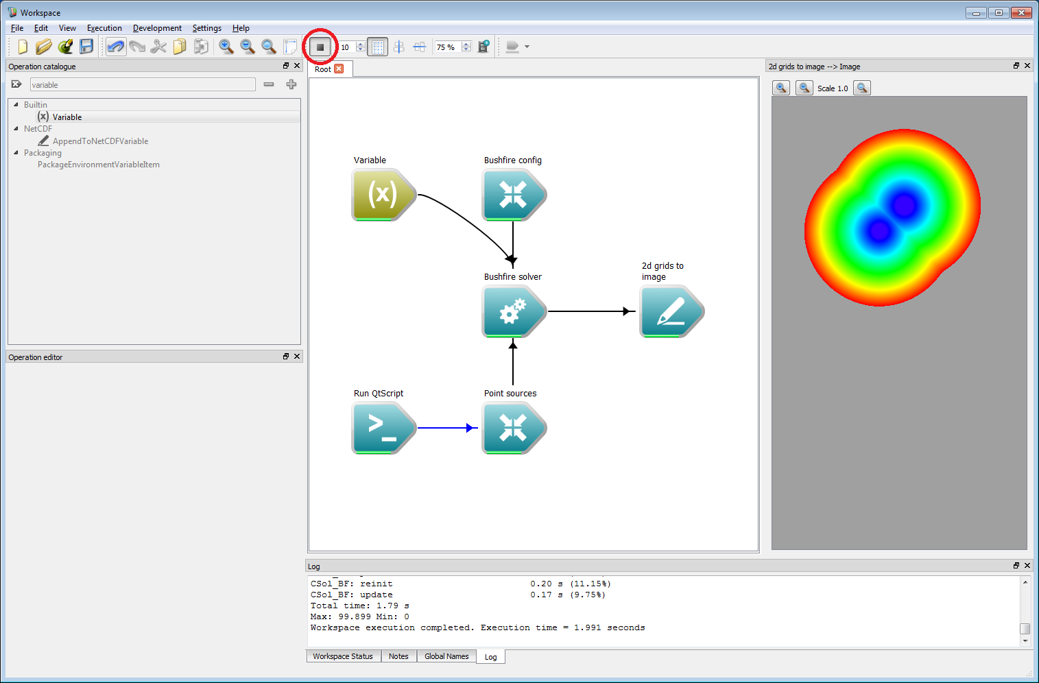Basic work-flow step 19

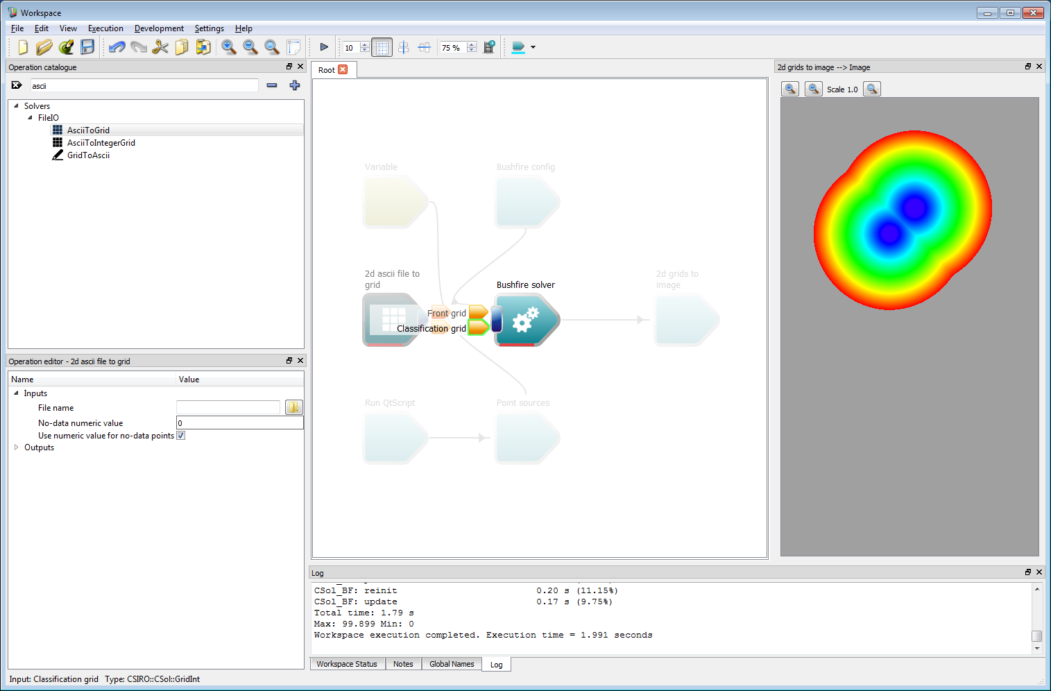
The output shows the arrival time of the two initial fire locations using a colur scale from blue (earliest time) to red (latest time). While this result looks interesting, there is still a short way to go to making this actually look like a realistic fire simulation.

Note
The speed function and script can be changed on-the fly which will cause the simulation to re-run and update.

To add another point, press the Toggle execution button to stop execution. Add another point in the script list and press the Toggle execution button to re-run.

Incorporating geospatial data

Example files.

The last example showed how a basic simulation can be constructed. This section will describe an example more applicable to realistic fires, albeit using some very synthetic data sets. All fuel and classification data sets have been prepared manually for this example and are only intended to be used as a guide for constructing more complex work-flows. Actual rate-of-spread models based on real data sets will be discussed in a future section.

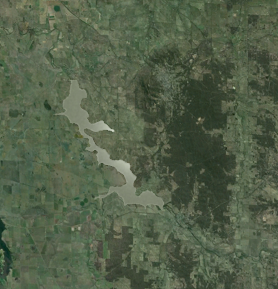
We will expand on the last example in the model. Firstly, we need to set the simulation time to a reasonable value. Click on the Bushfire config operation and set the Total simulation time and the Data write frequency inputs to 14,400 seconds (4 hours). Secondly, we need to set the tile size to a reasonable value. Click on the Bushfire solver operation and set the Tile size (power of 2) input to 7. This will make the tile size 2^7 = 128 units in size. The simulation will be run on an area of land around a reservoir in Victoria, an aerial image of which is shown below.

Incorporating geospatial data 1

Warning
Very large or small values of the tile size may cause issues on different operating systems and hardware. However, a value of 7 or 8 has been found to work best for most GPU or CPU set-ups.
The first data layer required is the classification layer. If this is not supplied, the solver assumes that all areas are burnable and sets the classification value everywhere to 1 (which also allows only one rate of spread model to be used). In this example, we use a classification of 0 (un-burnable) and a single fuel model with classification 1. The un-burnable areas in this simulation are simply water area of the reservoir. The classification layer is prepared as an ESRII ASCII data set. This can be converted to a Grid input layer using the AsciiToGrid operation. Add this operation to the work-flow and connect the Grid output to the Classification grid input of the Bushfire solver operation.

Incorporating geospatial data 2
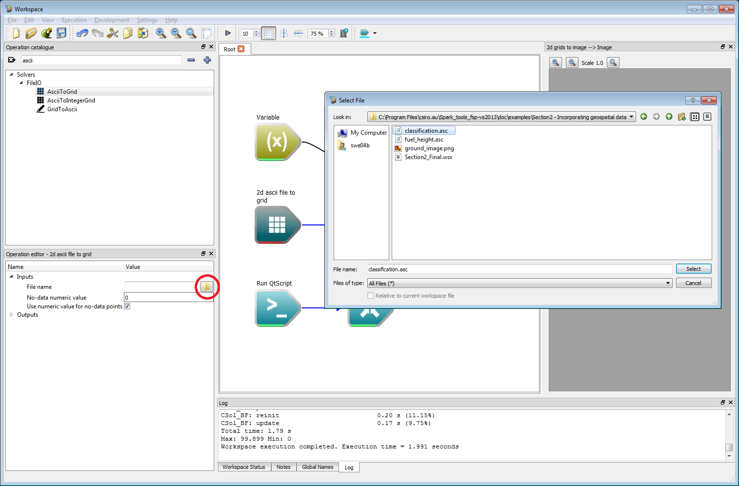
Select the AsciiToGrid operation and click on the open file button (circled red) within the operation editor. Select the classification.asc file from the set of example files.

Incorporating geospatial data 3
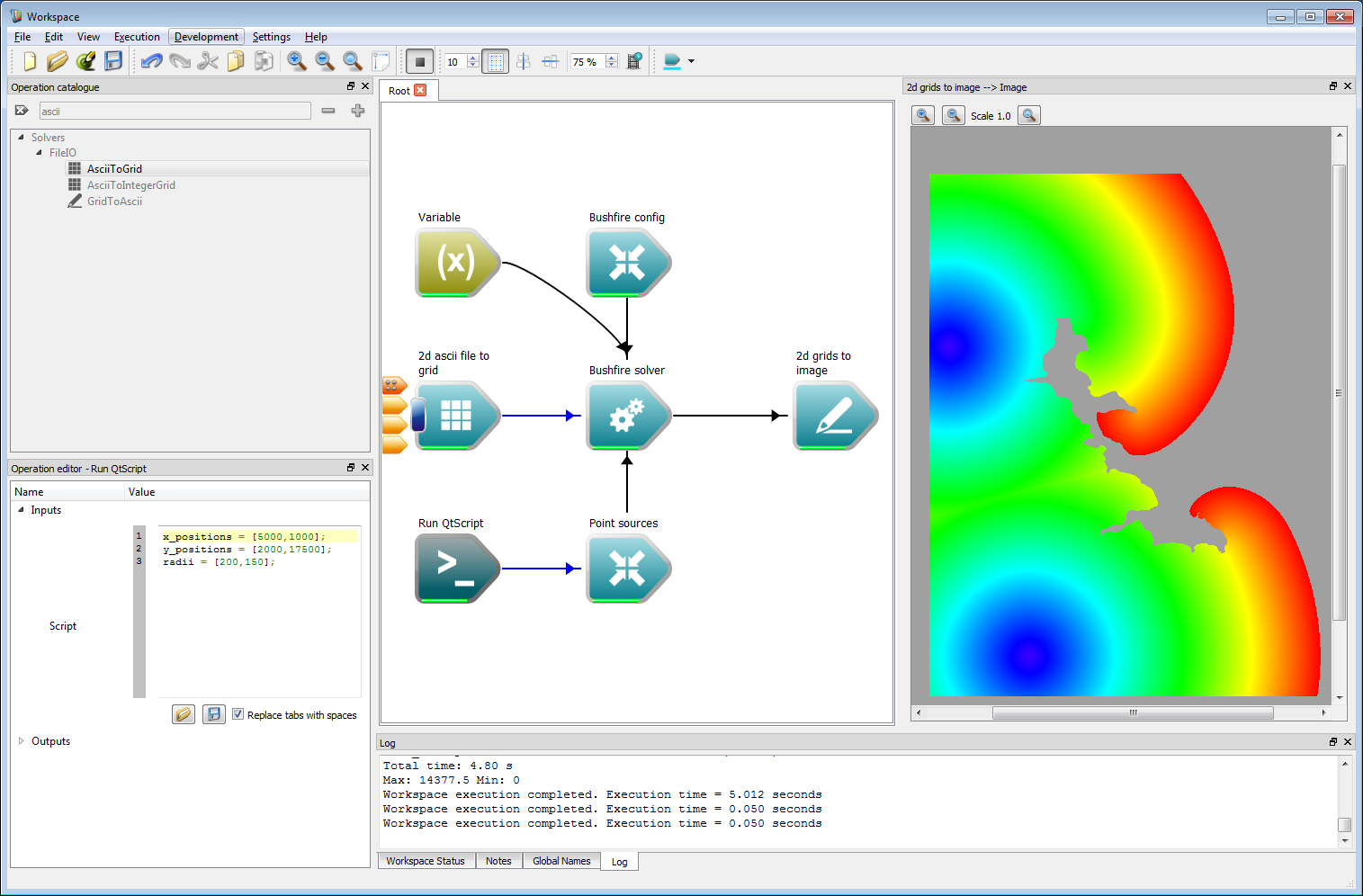
Change the resolutions used in the work-flow:
- Select the Point sources operation and change the Point source map resolution to 45 m.
- Select the 2d grids to image operation and change the Pixel resolution to 45 m.
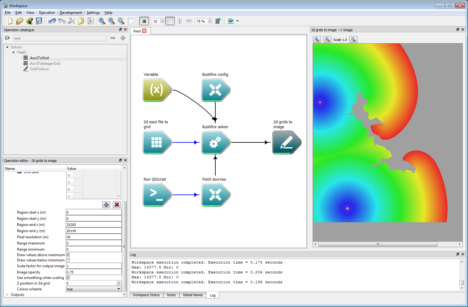
Also, change the point sources in the Point Sources script to the values:
x_positions = [5000,1000];

y_positions = [2000,17500];

radii = [200,150];

After setting these values, press the Toggle execution button to run the simulation. The resulting output should be the same as the figure below, showing a circular fire pattern spread around the un-burnable regions of the reservoir.

Incorporating geospatial data 4

Warning
Ensure that the pixel resolution is changed in the 2d grids to image operation, otherwise the image will be created at the previous resolution of 1 m, resulting in potential memory allocation failure.

Note
If a classification is provided, the cells outside the spatial limits of the classification region are assumed to be un-burnable. This prevents fires spreading beyond the regions for which classification data is provided.
The output image above can be processed as an overlay by imposing spatial limits. Also, the output settings can be tweaked to give a slightly better looking output. This can be carried out by selecting the 2d grids to image operation and carrying out the following steps:
- Change the region start location to 0 and 0 for x and y, respectively.
- Change the region end location to 25200 and 26145 for x and y, respectively.
- Uncheck the Draw values below minimum box.
- Set the image opacity to 0.75.
The output is the cropped and translucent image shown below.

Incorporating geospatial data 5

Note
The values given here are artificial, in more realistic application the start and end regions would be given by easting and northing values for a given zone.
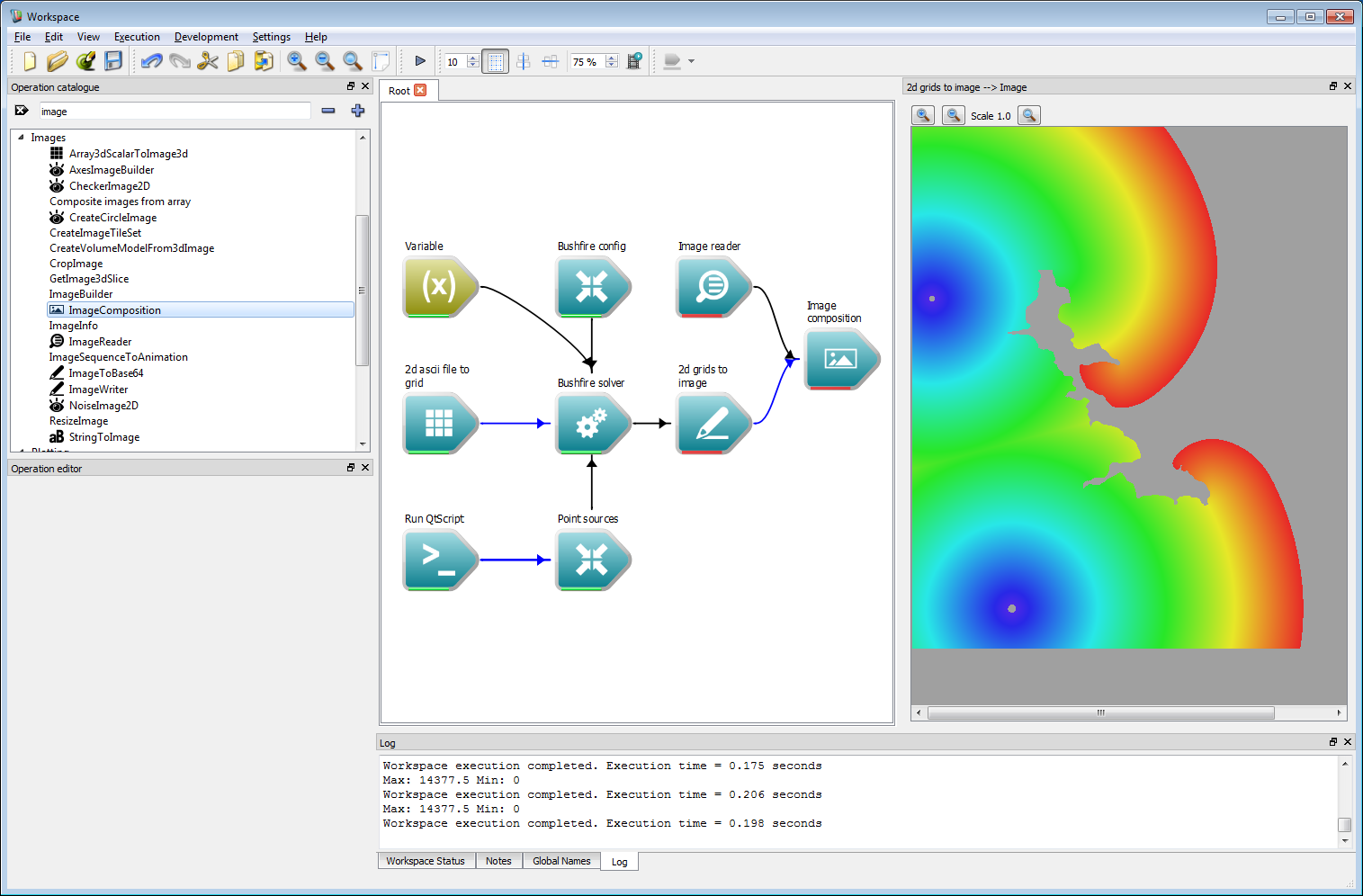
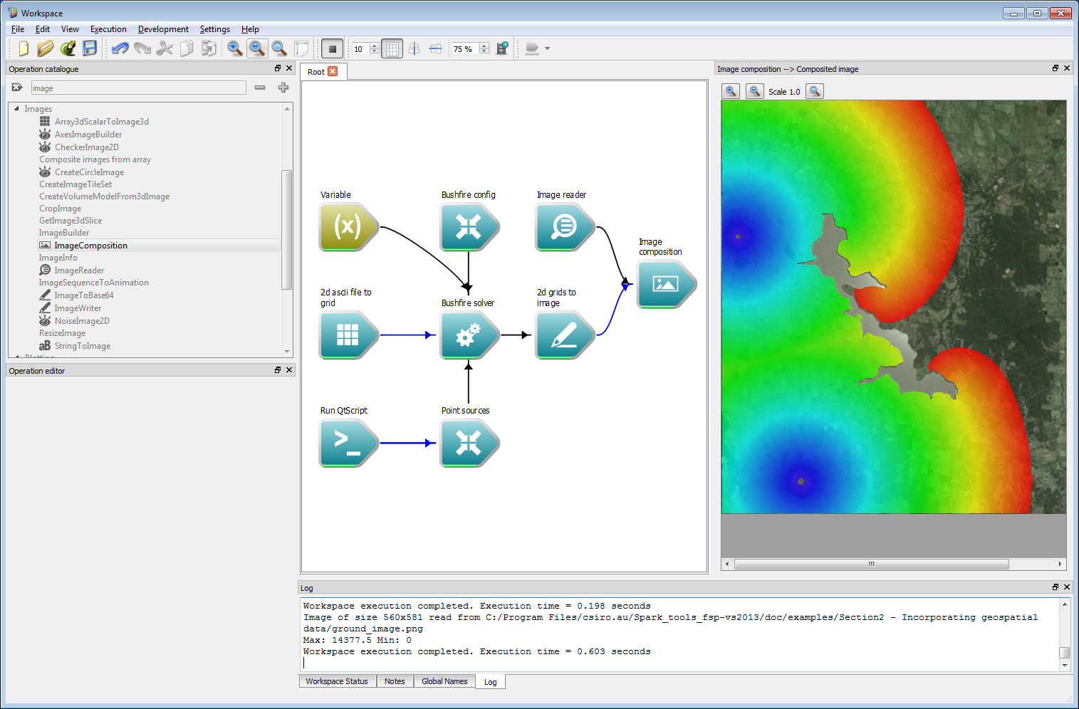
A backing plane can be added to show the fire location over a ground layer. To do this, add an Image reader operation and load in the required ground image. In this example, this is called ground_image.png. Next, add in an Image composition operation, and connect the Image output from the Image reader operation to the Base image input and the Image output from the 2d grids to image operation to the Image overlays input.

Incorporating geospatial data 6
Close the image display widget using the small 'X' in the upper right-hand corner and open a new image widget from the Composited image output of the Image composition operation. Executing the workflow will result in the image shown below.

Incorporating geospatial data 7

Note
Again, the use of a pre-defined base plane is for this artificial example. Layers projected onto interactive maps will be discussed later.
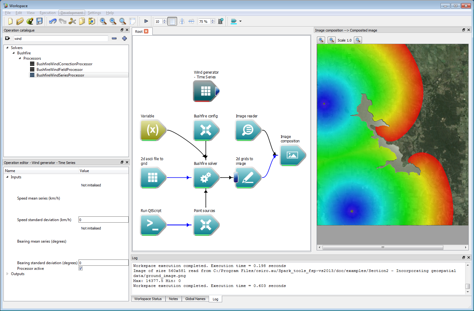
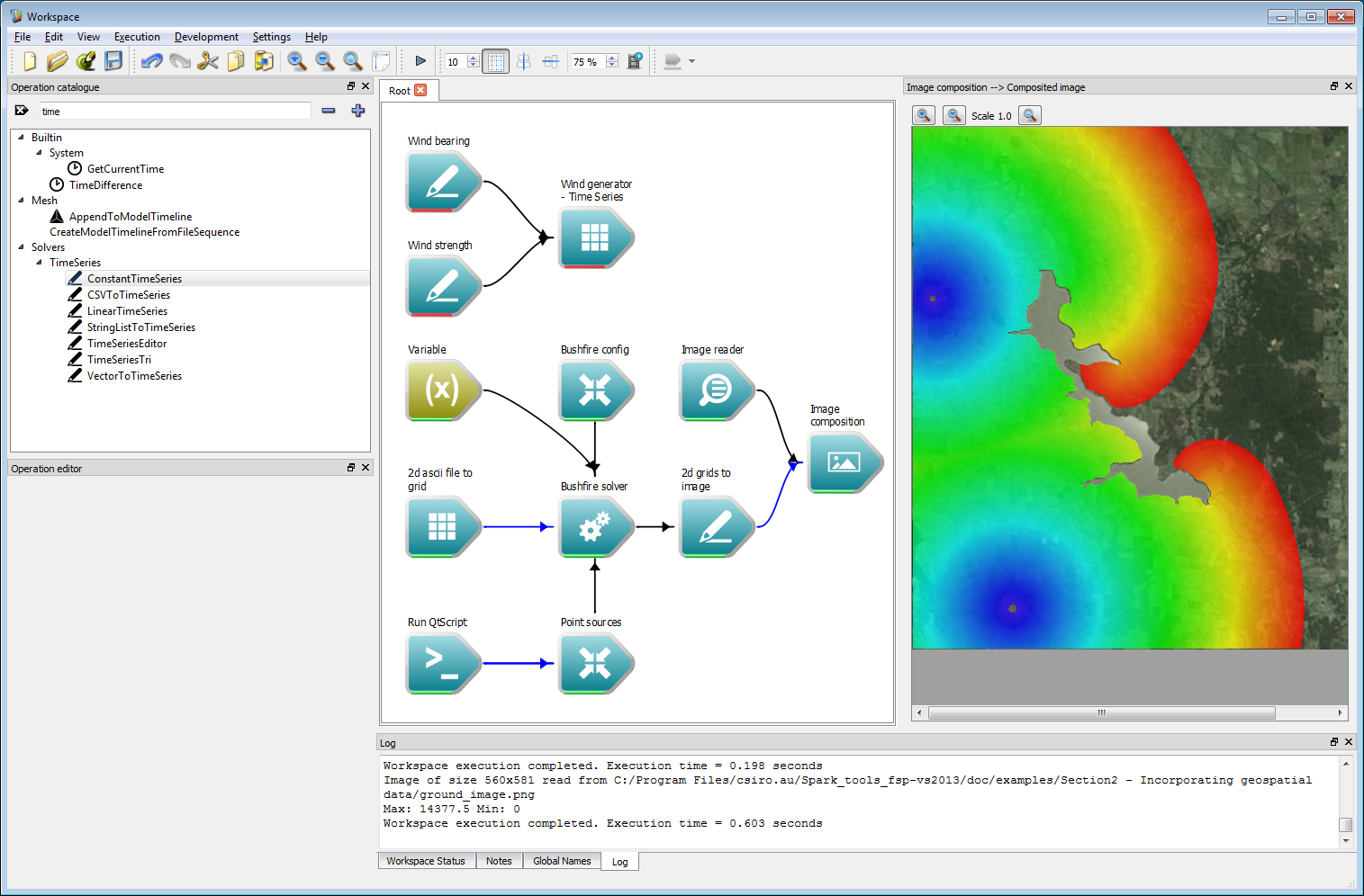
Wind is the primary driving factor for bushfires. Wind can be imposed in a number of ways in Spark, the simplest being a time-series operation. Create a BushfireWindSeriesProcessor. This takes two inputs, a wind strength input and a wind bearing input.

Incorporating geospatial data 8
The time-series can, again, be incorporated in a variety of ways. This includes constant, linear and variable data streams from inputs such as CSV files. Here, we will use a constant time-series which is implemented using the ConstantTimeSeries operation. Create two constant time-series operations and label them Wind bearing and Wind strength. Set the wind bearing value to 220 degrees and the wind strength to 10 km/h. Connect these two operations to the corresponding Bearing mean series and Speed mean series inputs of Wind generator - Time Series operation.

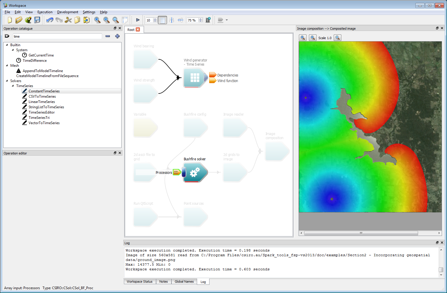
Incorporating geospatial data 9
Connect the Wind generator - Time Series operation to the Processors operation of the Bushfire solver operation. Processors are sub-solvers which run independently of the solver at each time-step. This wind processor generates a wind field that is used by the solver.

Incorporating geospatial data 10
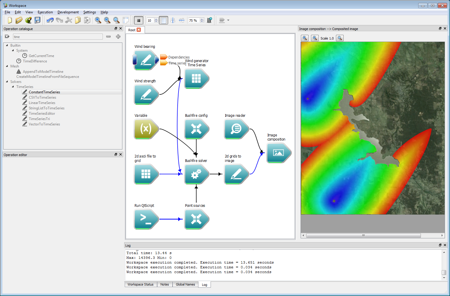
Next, the rate-of-spread model can be changed to be a bit more interesting. In this example we have changed it to use a constant rate of spread plus a term that depends on the square of the wind parameter. This wind parameter is defined as the dot product of the wind vector in each cell and the vector normal to the fire front, with a minimum value of zero. The example rate of spread model used here is:
speed = 0.5+0.02*wind*wind;

Running the simulation now shows a strong wind dependency.

Incorporating geospatial data 11

Note
Any OpenCL C mathematical functions are allowed in the speed function definition.
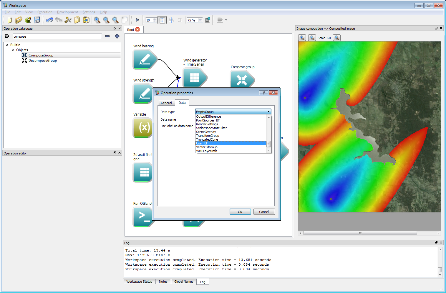
The fire propagation rate given in the code above, based by a constant multiplied by a function of the wind speed, is not particularly suitable for a usable fire model. Fire models typically depend on many spatially and temporally varying parameters, such as fuel condition, temperature and moisture levels. Such user-defined spatial layer can easily be added and used in rate-of-spread models. First, create a Compose Group with a data type of User_BF.

Incorporating geospatial data 12
This user layer will store a value for fuel height. The Compose Group operation has been labelled Fuel Layer in the example shown below. Next, create a AsciiToGrid operation and set the operation to load a fuel data file, called fuel_height.asc in this example. Connect the Grid output from the AsciiToGrid operation to the User data grid input of the Fuel Layer operation.

Select the Fuel Layer operation and enter 'fuel_height' as the User data name. This will be the name that the user layer is referred to in the speed function. The fuel layer also allows a randomisation initialisation around a normal distribution of a given width of User data variation. Values outside the spatial range of the input layer are set to the User data external value. In this example the external data value is zero, meaning that any fuel height values outside the spatial range of the original ESRII ASCII data layer are considered to be zero.

Incorporating geospatial data 13

Note
Any number of user data layers are allowed, provided they have unique names. The variables defined from each layer can be used in the speed function. For example, if user data layers temperature, relative_humidity and fuel_load are defined the speed function could be a statement such as: speed = 0.1*fuel_load+0.3*pow(temperature, 0.25)*relative_humidity.
Connect the Object group output from the Fuel layer operation to the User data grids input of the Bushfire solver operation.

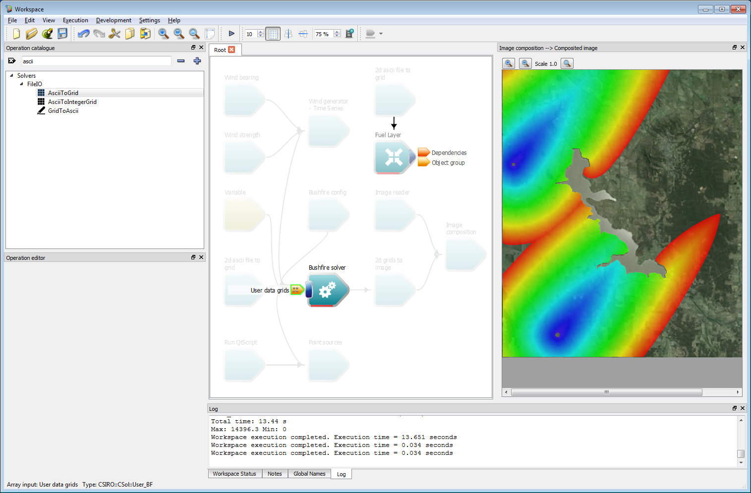Incorporating geospatial data 14
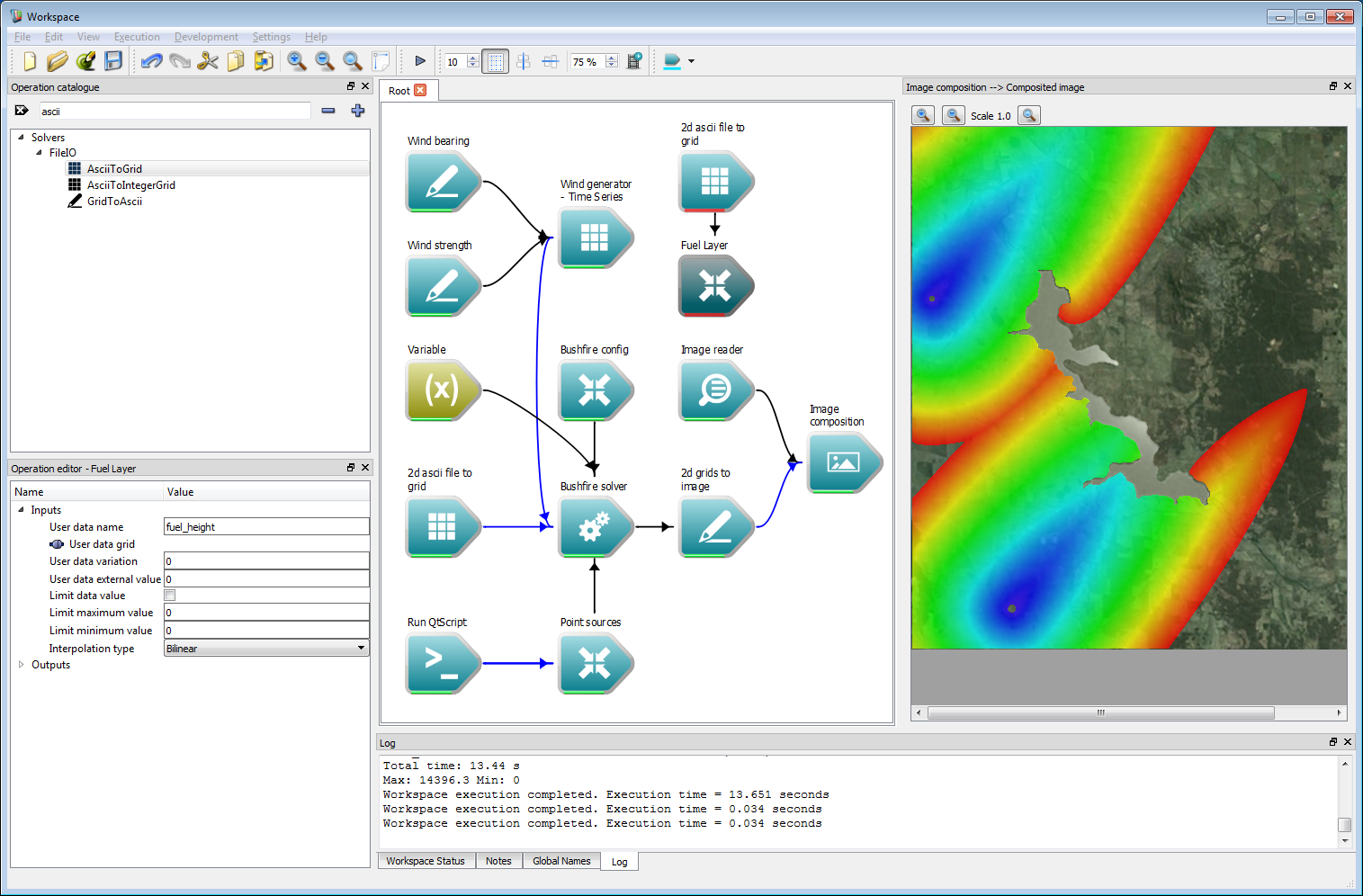
The rate-of-spread model can now be modified to use this user data layer. The resulting output from the modified rate-of-spread model:
speed=0.005*fuel_height+0.01*wind*wind;

is shown in the figure below.

Incorporating geospatial data 15

Note
Any inputs can be shown in their own window, such as the rate of spread string. To do this, right-click on the corresponding input and select a widget type from the menu. For the rate-of-spread model, right click on the QString input of the Rate-of-spread model variable and select Display with QTextEdit.
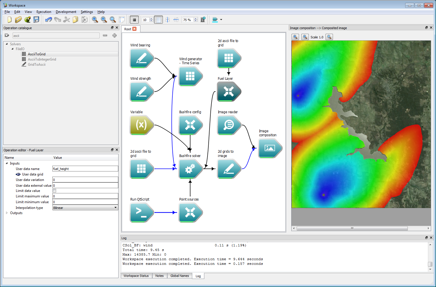
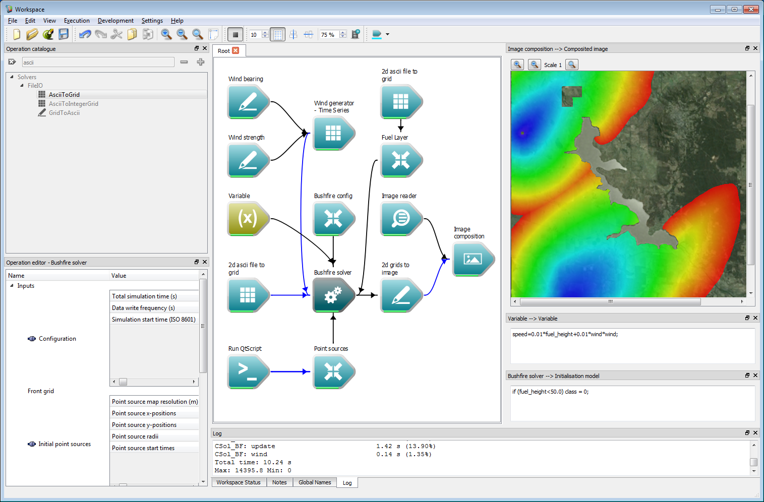
Finally, an initialisation model can be executed on the data layers before the simulation is started. This uses the Initialisation model input on the Bushfire solver operation. This model can read and write to any of the user defined data layers, or the classification layer. For example, regions where the fuel height is less than 50 cm is set to un-burnable using the initialisation model:
if (fuel_height<50.0) class = 0;

There is a region to the north of the reservoir where this is the case in the example, and the resulting output is below.

Incorporating geospatial data 16

Interactive control

Example files.

The previous example ran a simulation a single time and displayed the result. In some instances, it may be preferable to display the results interactively for debugging or visualisation. Spark allows control to be returned to the work-flow after a specified amount of time allowing visualisation, sampling or other analysis steps of the data as it is generated. This is implemented using a loop system within the work-flow.

Search for the While loop operation in the catalogue and add it to the work-flow.

Interactive control 1
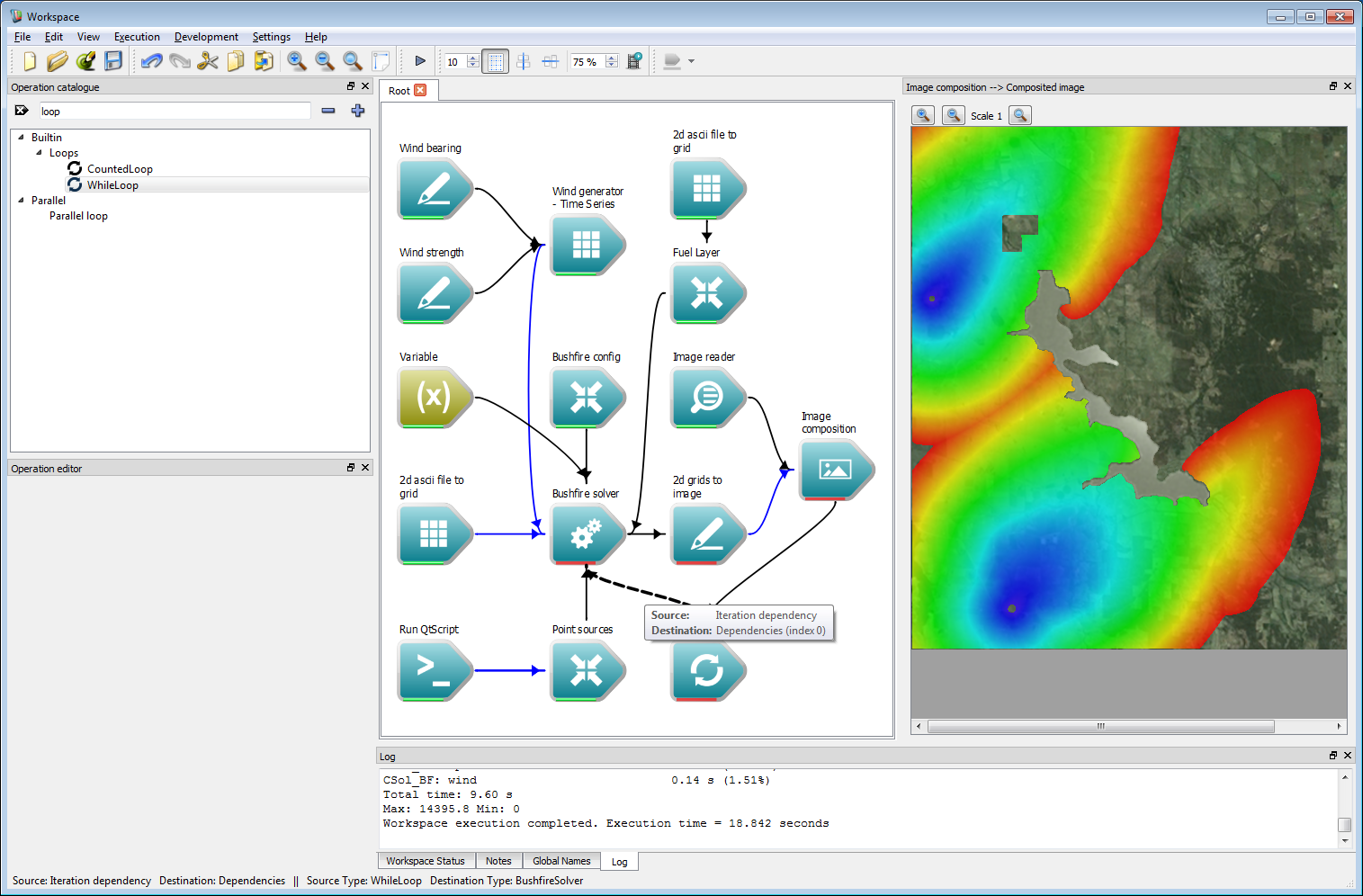
Connect the Dependencies output of the Image composition operation to the Iteration dependency input of the While loop operation. Connect the Iteration dependency output of the While loop operation to the Dependencies input of the Bushfire solver operation.

Interactive control 2
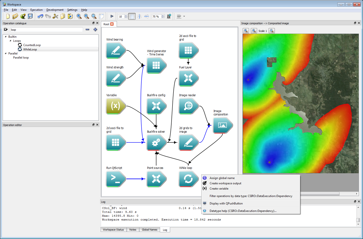
The work-flow now needs a global end-point. This can be created by right-clicking on the Dependencies output of the While loop operation and selecting Create workspace output.

Interactive control 3
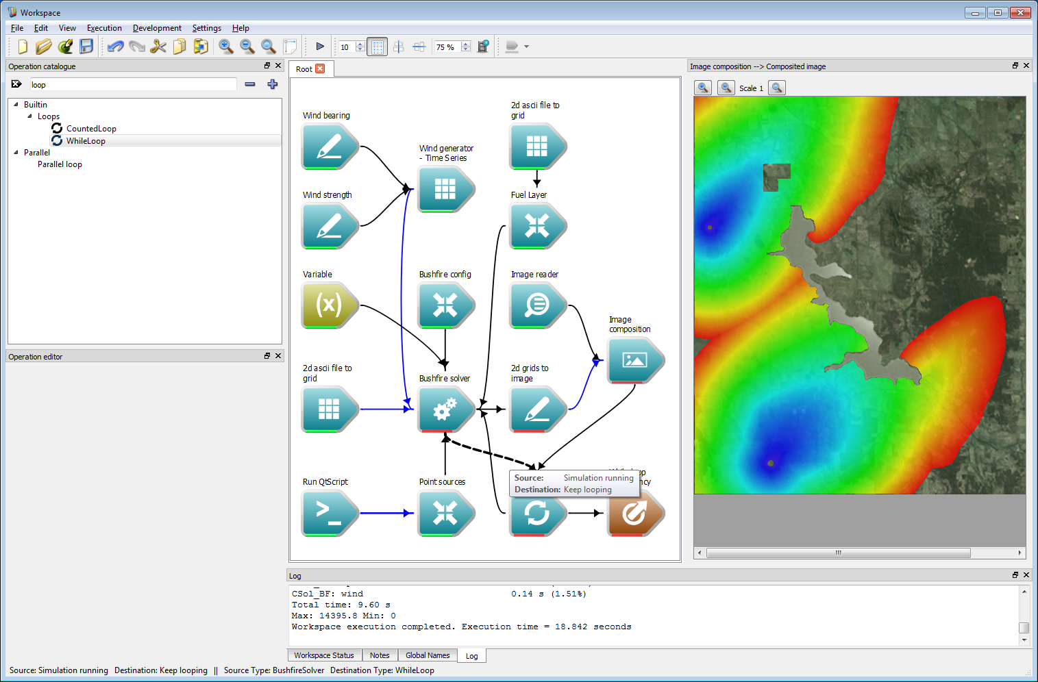
The while loop needs a signal to stop. Connect the Simulation running output of the Bushfire solver operation to the Keep looping input of the While loop operation.

Interactive control 4
Lastly, choose the period of time between outputs. Select the Bushfire config operation and set the Data write frequency to 1,800 s, keeping the total simulation time at 14,400 s.

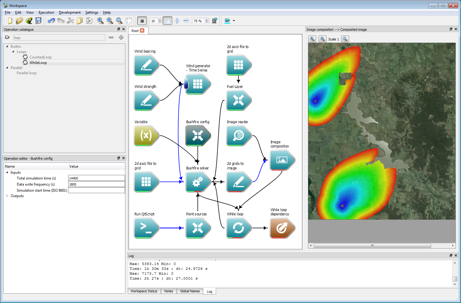Interactive control 5

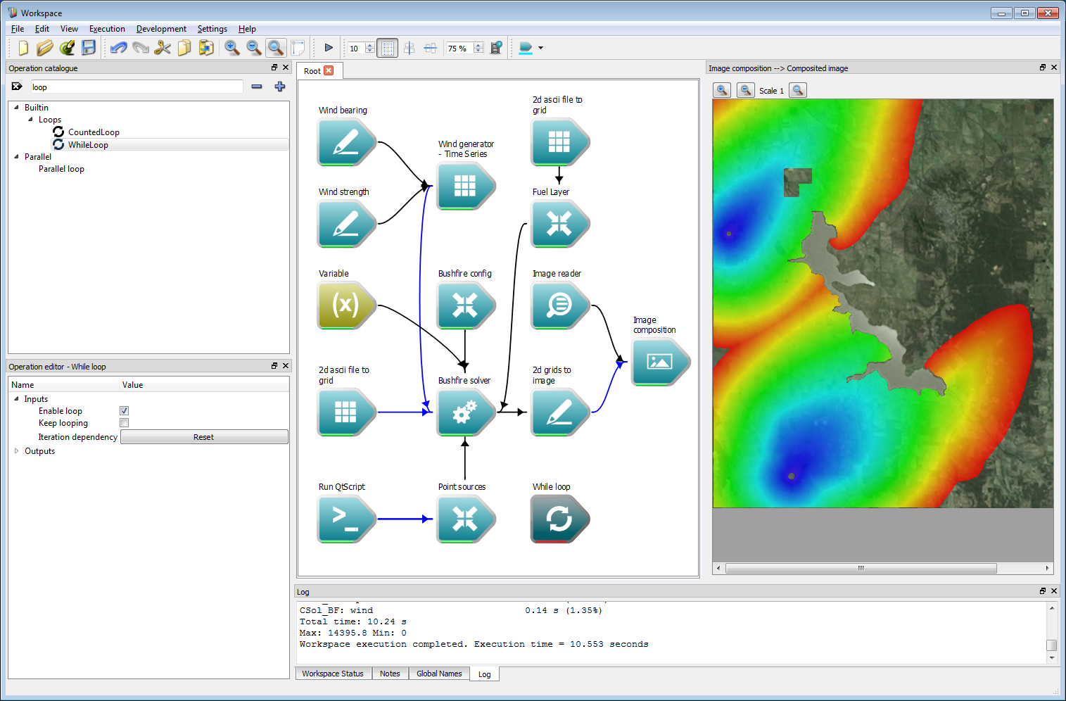
Running the simulation will now give an animated output.

Ensemble analysis

Example files.

Running a single simulation presents only a single possible outcome depending on many varying factors. For risk analysis (and even operational usage) multiple simulations present a more complete picture of the potential outcomes of a fire scenario. Creating such ensemble simulation within Spark is very straightforward using the built-in Workspace looping mechanisms.

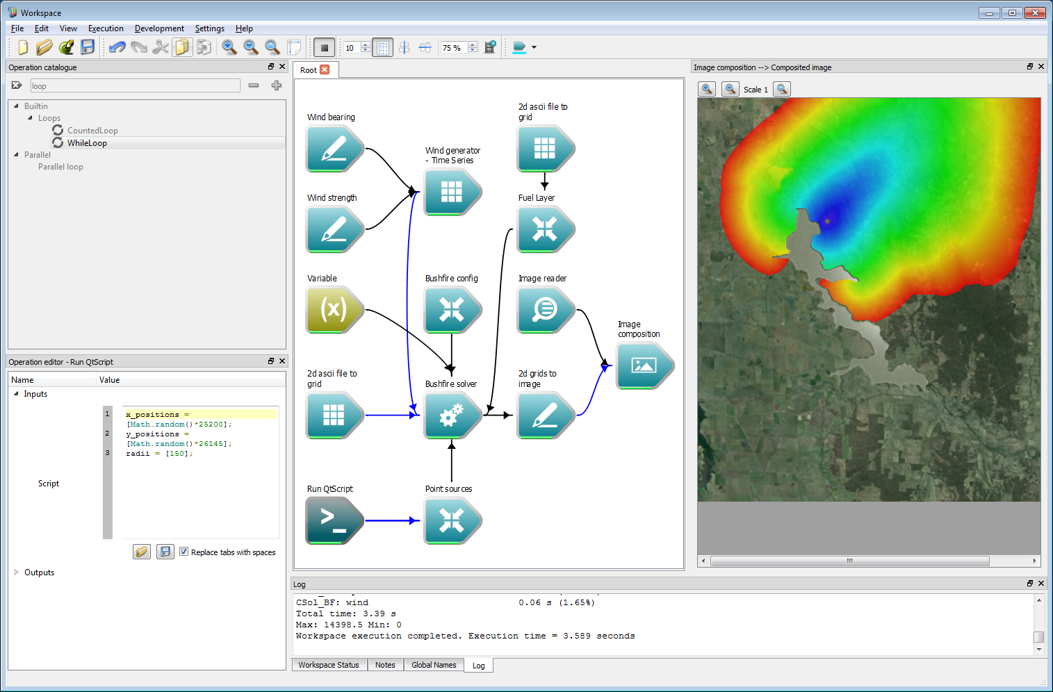
First, we need a simulation with a random outcome. It is easiest to modify the existing work-flow from the previous example. Firstly, we will need to remove the while loop as this will be replaced later with a loop over the number of events in the ensemble. Select the While loop operation and press the DELETE key to remove it. Remove the While loop dependency in the same way. Next, select the Bushfire config operation and change the Total simulation time and Data write frequency to the same value of 14,400 seconds. To start a fire at a random location change the code in the Run QtScript operation to the following:
x_positions = [Math.random()*25200];

y_positions = [Math.random()*26145];

radii = [150];

The function Math.random() returns a random value for 0-1 which is multiplied by the spatial range of the domain. Running the simulation will start a fire at a random point within the domain. To re-run the simulation, right-click on the Run QtScript and select Reset operation.

Ensemble analysis 1

Warning
Ensure that both the Total simulation time and Data write frequency are equal, or the simulation will end after the Data write frequency time has elapsed.

Note
If a starting point is within an un-burnable region the simulation is simply ended.
To keep track of the number of simulations, add a new input to the Run QtScript operation. Double click on the operation and add a new input called count. This will hold the index of the simulation in the ensemble.

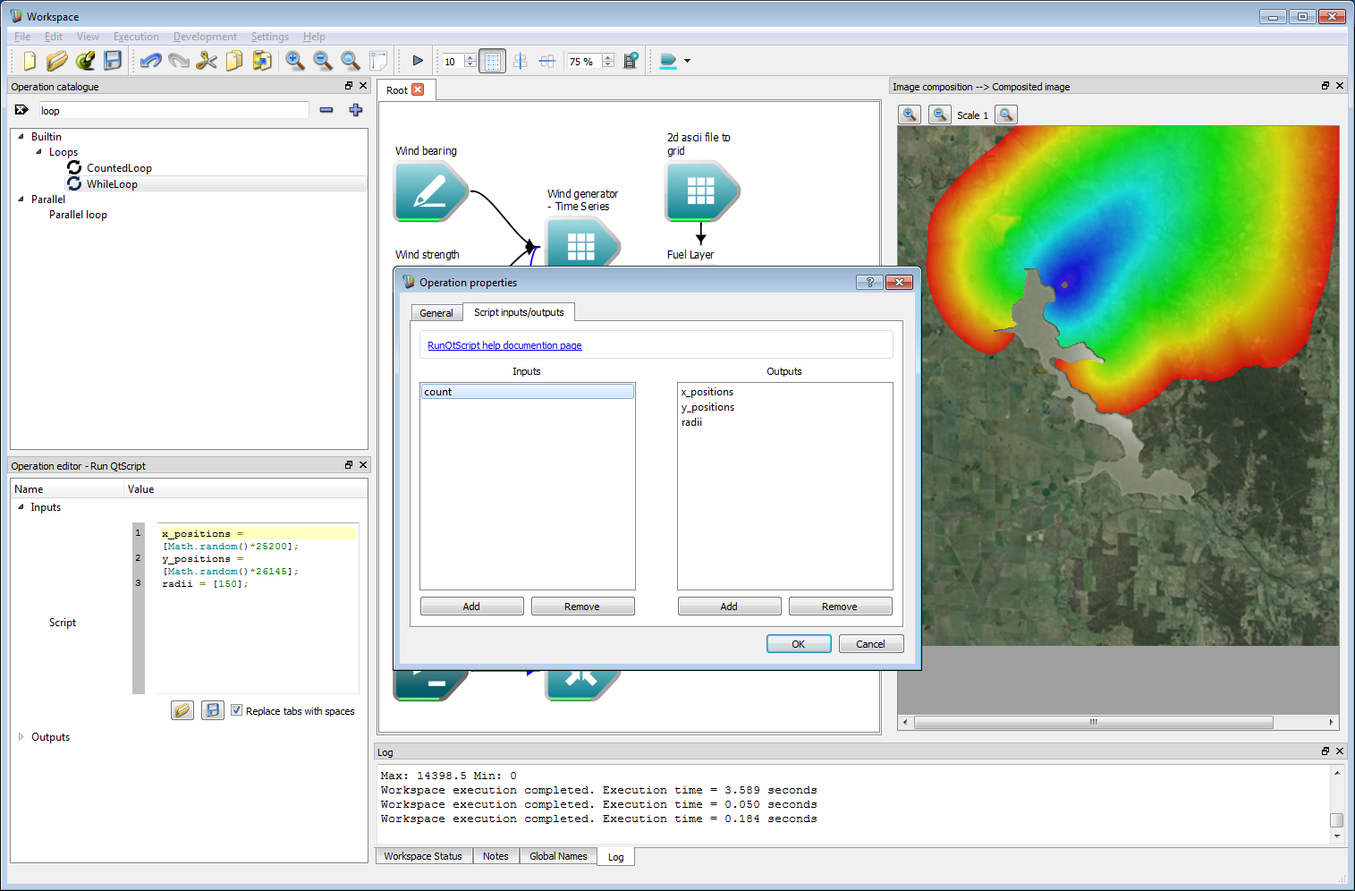Ensemble analysis 2
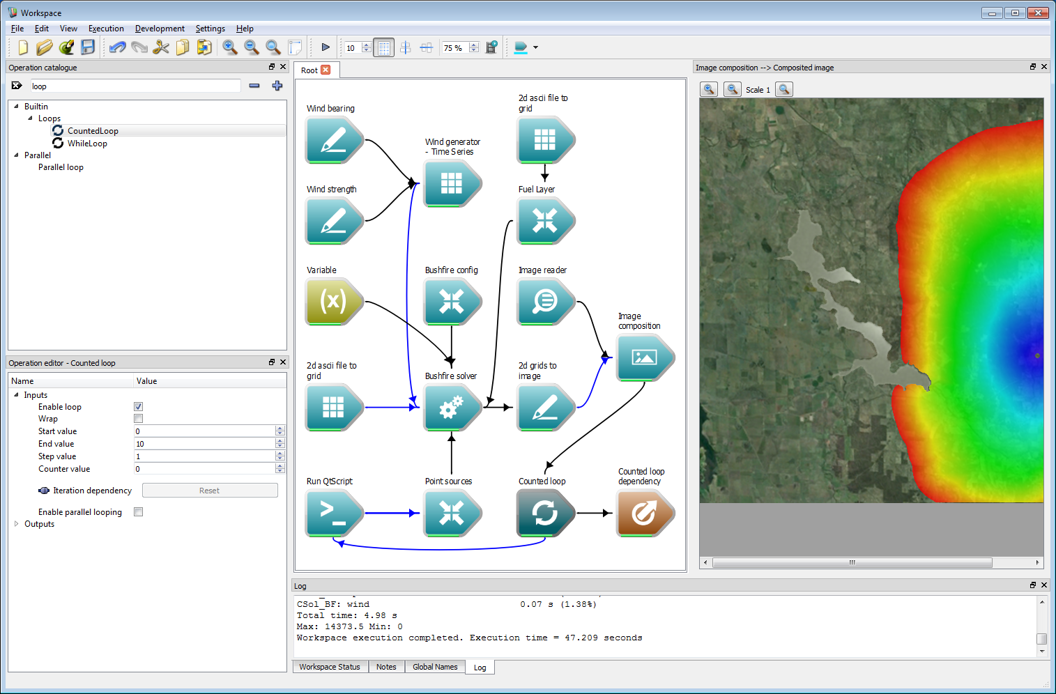
Create a Counted loop operation and add a global end-point by right-clicking on the Dependencies output of the Counted loop operation and selecting Create workspace output. Connect the Dependencies output of the Image composition operation to the Iteration dependency input of the Counted loop operation. Connect the Counter value output of the Counted loop operation to the new count input of the Run QtScript operation. Select the Counted loop operation and set the End value to 10. Executing the work-flow will run ten simulations with ten fires starting in different places.

Note
If ten different outputs do not appear, ensure that the Total simulation time and Data write frequency are equal to the same value.

Ensemble analysis 3
Before carrying out any ensemble operations we need to convert the tiled output from the solver into a single raster layer. This is done using the Grid Composite operation which joins any number of Grids into a single Grid. The spatial spacing and region in the output Grid can be specified, along with thresholding options for the spatial grid values. Add a GridComposite operation to the work-flow and check the Replace null data box. Set a value of -1 for the Replace null data value. The arrival time layer is set to a no-data value outside tiles containing the fire perimeter. This option will overwrite these no-data values with a value of -1, indicating regions outside the fire perimeter. Next, check the Use region box and input the spatial region used for the example data. This is a maximum of 25200 m in x and 26145 m in y. Connect the Arrival time Grid output from the Bushfire solver operation to the Input grids input of the Grid Composite operation. Select the 2d Grids to Image operation and press delete to remove the operation.

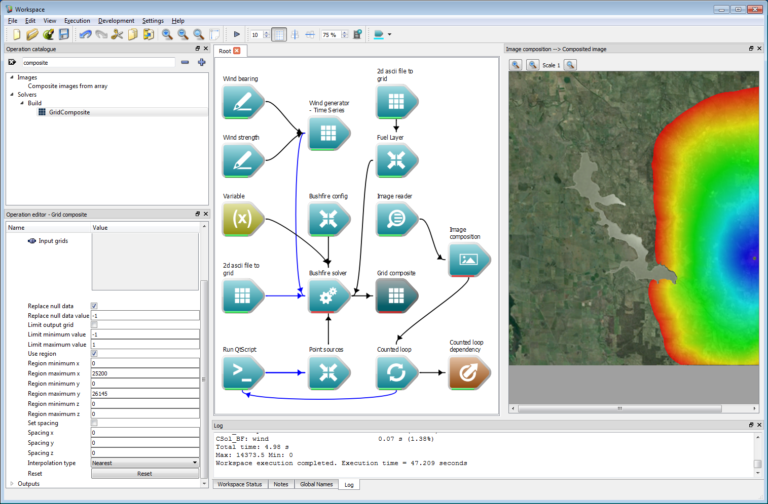Ensemble analysis 4

Warning
Ensure both the Replace null data box and Use region box are checked or the resulting data will appear incorrect.
We need a way to keep track of spatial layer values over multiple simulations. Spark provides a generic operation called a Grid operator which can hold an internal spatial layer that accrues values over multiple iterations. The operation allows a range of mathematical operations over a data layer. Add a Grid operator operation (called GridOperator) and connect the Output grid output of the Grid Composite operation to the Grid A input of the Grid operator operation. Select the Grid operator operation and choose the Maximum operation from the drop down Type list. This will compare each raster cell value to the previous raster cell, replacing the previous value if the new value is higher. Create a new image viewing operation using a 2d grid to image operation (note this is the singular 'grid' version) and connect the Result R output of the Grid operator operation to the Grid data input of the 2d grid to image operation. Untick the draw values below minimum option in the 2d grid to image operation. Connect the image output from the 2d grid to image operation to the Image overlays input of the Image composition operation. Finally, run the work-flow. The multiple simulations will now on a single image, which will be built up as each simulation runs.

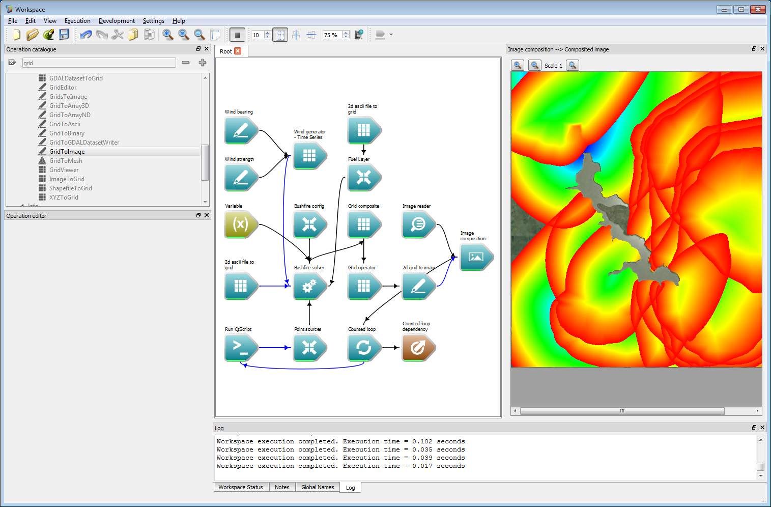Ensemble analysis 5

Note
For several functions the 'operator' operation uses two inputs, A and B. If A and B are both given, the operation uses A and B to produce the result. If only A is given, as is the case here, the operation uses an internal spatial layer called R to produce the result.

The Grid operator operation also supports running a script on each point in the layer for maximum flexibility. This is much slower than the pre-set operation types, however.
The maximum operation in the previous step could be used, for example, to store the maximum radiant heat flux from a number of fire simulations. Another option is to count the number of randomly started fires that arrive at a particular location. This can be done with one extra operation which converts the values of the arrival time layer to zero if un-burnt and one if burnt. These can be added to give the required count. Change the Type in the Grid operator operation from Maximum to Add. Remove the link between the Grid composite operation and the Grid operator operation by right-clicking and selecting Remove connection Add a Grid threshold operation, connecting the Output grid of the Grid composite operation to the Grid A input of the Grid threshold operation. Connect the Result R output of the Grid threshold to the Grid A input of the Grid operator operation. Select the Grid threshold operation and set the Threshold value to -1, the Threshold comparison to Greater than, check the overwrite data if threshold met option and set the Overwrite value to 1. These values are shown in the operation editor panel in the image below. These threshold values will set all values not meeting the threshold to zero, and (in this case) overwrite values meeting the threshold with one. Re-running the work-flow will give an output similar to the figure below, where the colour scale represents the number of simulations predicting fire perimeters encompassing any raster cell, with red the highest and blue the lowest.

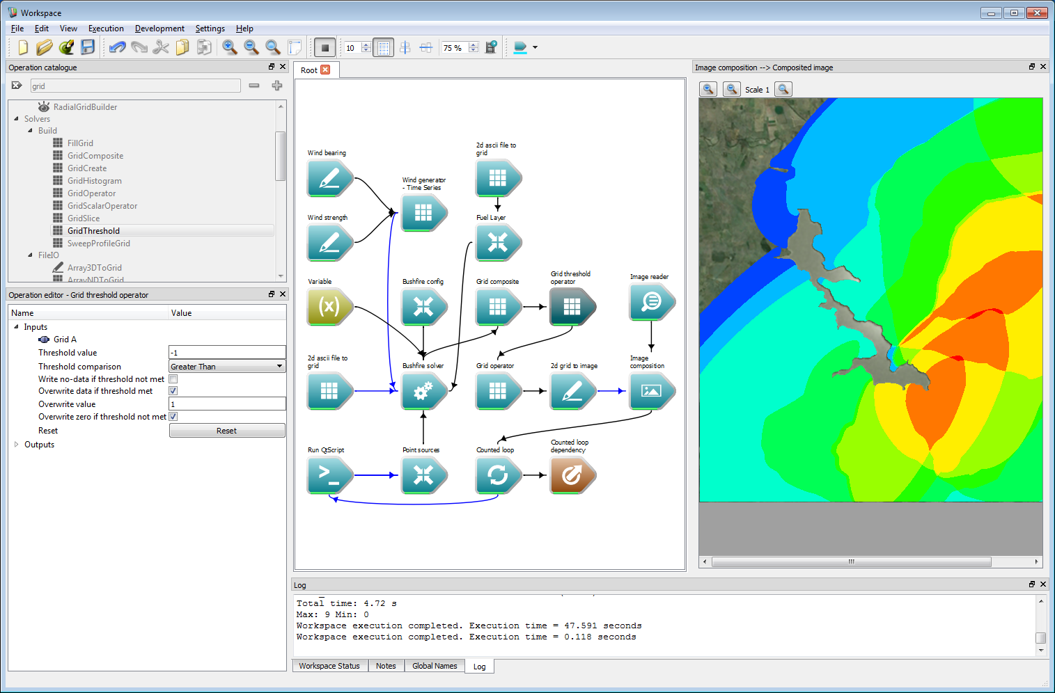Ensemble analysis 6

Note
The maximum and minimum rages for the image are output to the log. Here red corresponds to a count of 9 and dark blue corresponds to a count of 0.
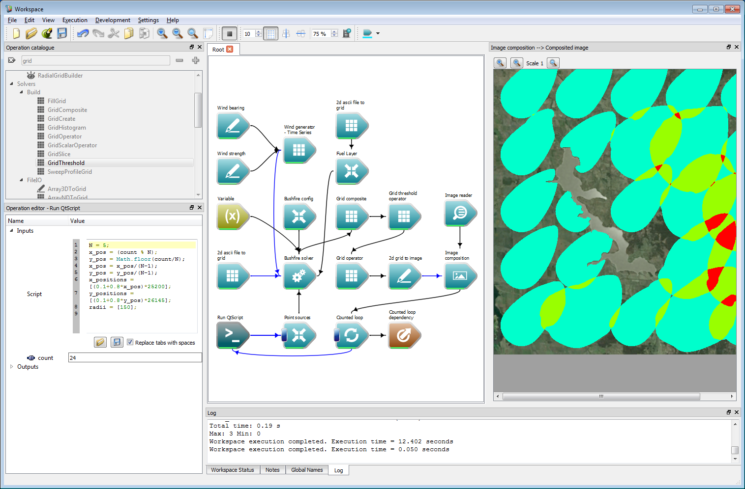
Of course, the simulations do not have to be randomly placed. The script can easily be set to run over a regularly spaced grid, as shown in the figure below. The code in the script used for this was:
N = 5;

x_pos = (count % N);

y_pos = Math.floor(count/N);

x_pos = x_pos/(N-1);

y_pos = y_pos/(N-1);

x_positions = [(0.1+0.8*x_pos)*25200];

y_positions = [(0.1+0.8*y_pos)*26145];

radii = [150];

This was run over 25 simulation, where N is the square root of the number of simulations. Note that the simulation time for each simulation was set at an hour in this example. The colour scheme has also been changed from the simulations used in the previous step. Any set of starting locations required can be programmed and provided to the simulations in such a manner.

Ensemble analysis 7

Note
To re-run the ensemble simulations using a different script the Grid operator and Counted loop operation must be reset by right-clicking when the work-flow is running and selecting Reset operation. For complex work-flows it is sometimes easiest to save and re-open the work-flow to ensure all operations are fully reset.

Geospatial integration

Example files.

The Spark framework supports reading and writing a wide range of raster and vector formats. Raster formats are handled using GDAL, which can be read and written directly to Grid layers. The main vector format used by Spark is the ESRI shapefile, although VTK files can also be used if required.

GDAL compatible files can be read using the OpenGDALDataset operation, where the type of file is inferred from the file extension. ESRII ascii, NetCDF and GeoTIFF formats have all been fully tested, although the operation should be able to use any supported GDAL data type. The GDALDatasetToGrid operation is used to convert the GDAL dataset to a internal Grid layer. If the underlying data has a time dimension (such as gridded weather data), this is stored in the third, z, dimension of the internal Grid. The z dimension is used as time in this case, and the spacing between the z layers is given by the time-step between each time slice in the data. This time step is detected for NetCDF files by searching for NETCDF_DIM_time_VALUES in the metadata. If this is found, the Data start time output of the operation is also set. The example below shows the output from reading a NetCDF file for elevation in the Blue Mountains region in NSW.

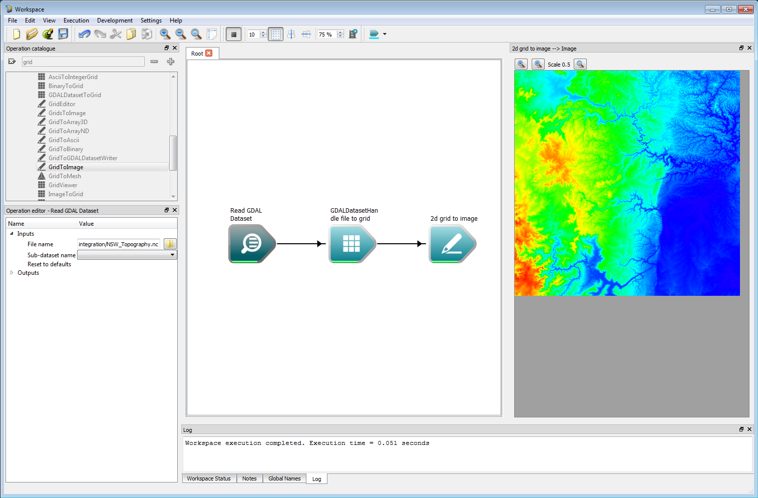Geospatial integration 1
Before using the data in a simulation, it needs to be re-projected. Spark uses Cartesian grids equispaced in meters for calculations, so a UTM projection is ideal. For efficiency, Spark contains an operation GeospatialProjection to convert between common projects such as lat/long and Australian MGA. The operation requires OGC Well Known Text (WKT) strings for the input and output projections. After conversion, the Grid is correctly scaled in a Cartesian system suitable for use.

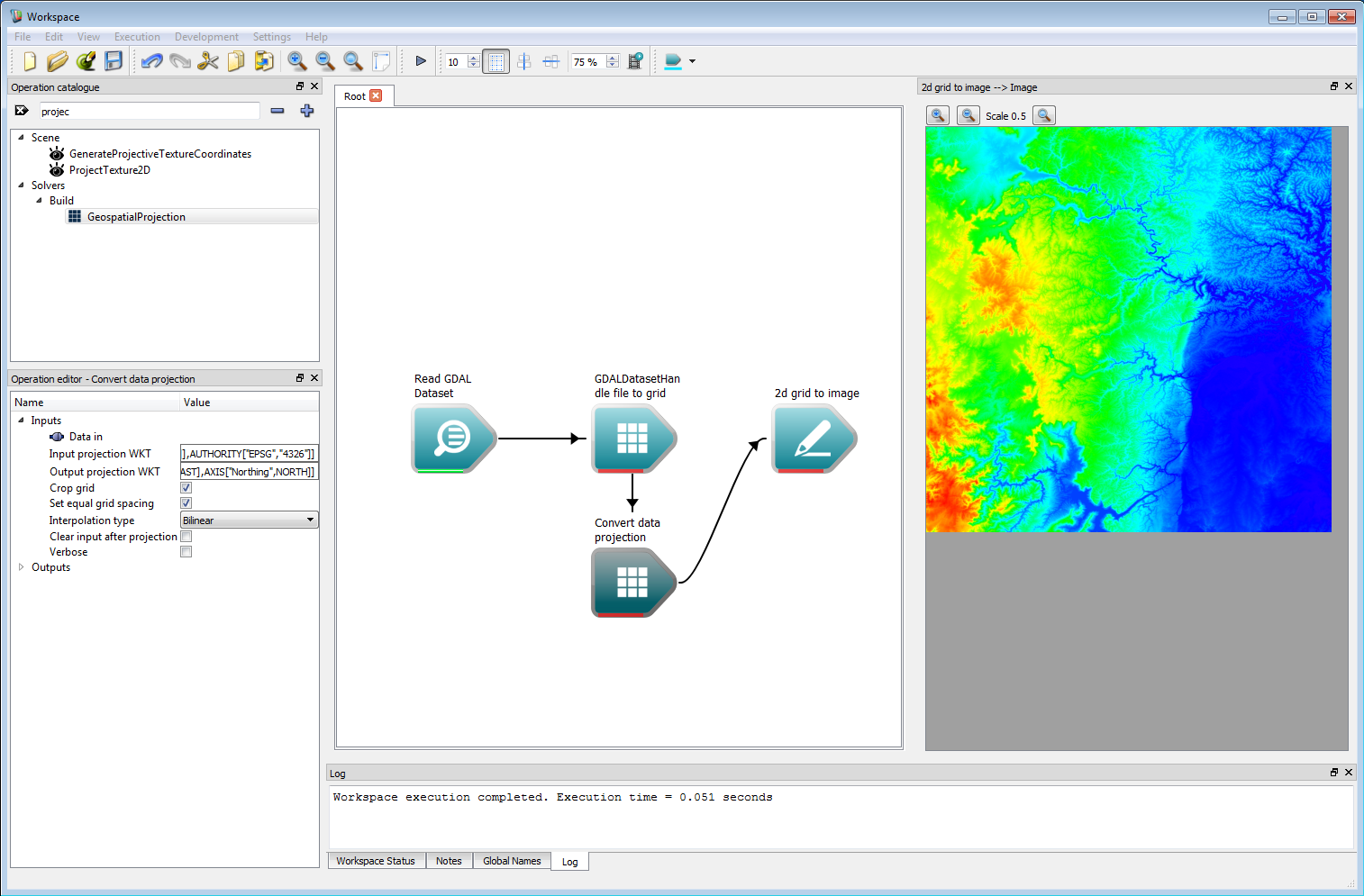Geospatial integration 2
Spark contains an interactive map widget through the Workspace geospatial system. Creating a raster layer on this map requires a CreateImageMapLayer operation. This operation takes an Image as input as well as a geospatial bounding box. This bounding box can be created using a Grid to Geospatial Bounding Box operation.

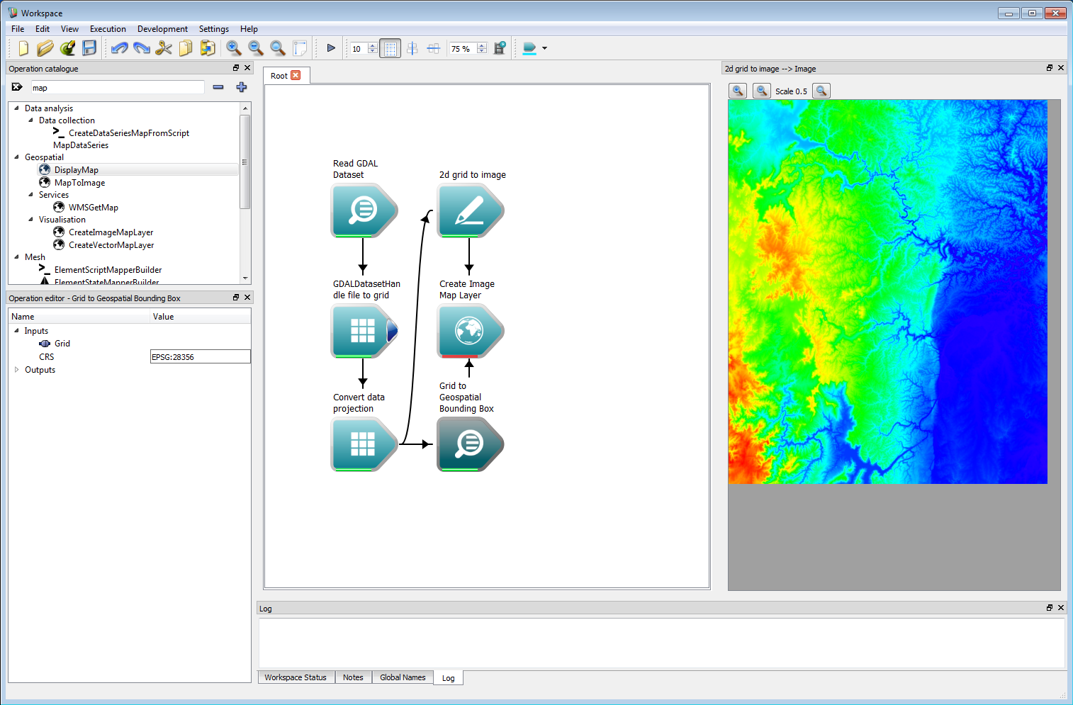Geospatial integration 3
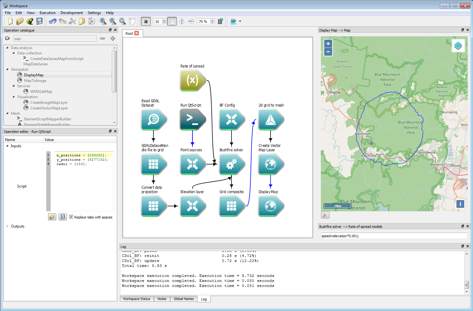
Once all these connections have been made, the DisplayMap operation can be used to show an OpenLayers map for the region. Right-clicking on the Map output of the Display Map operation and selecting Display with MapWidget will show the map in a widget which can be docked with the canvas.

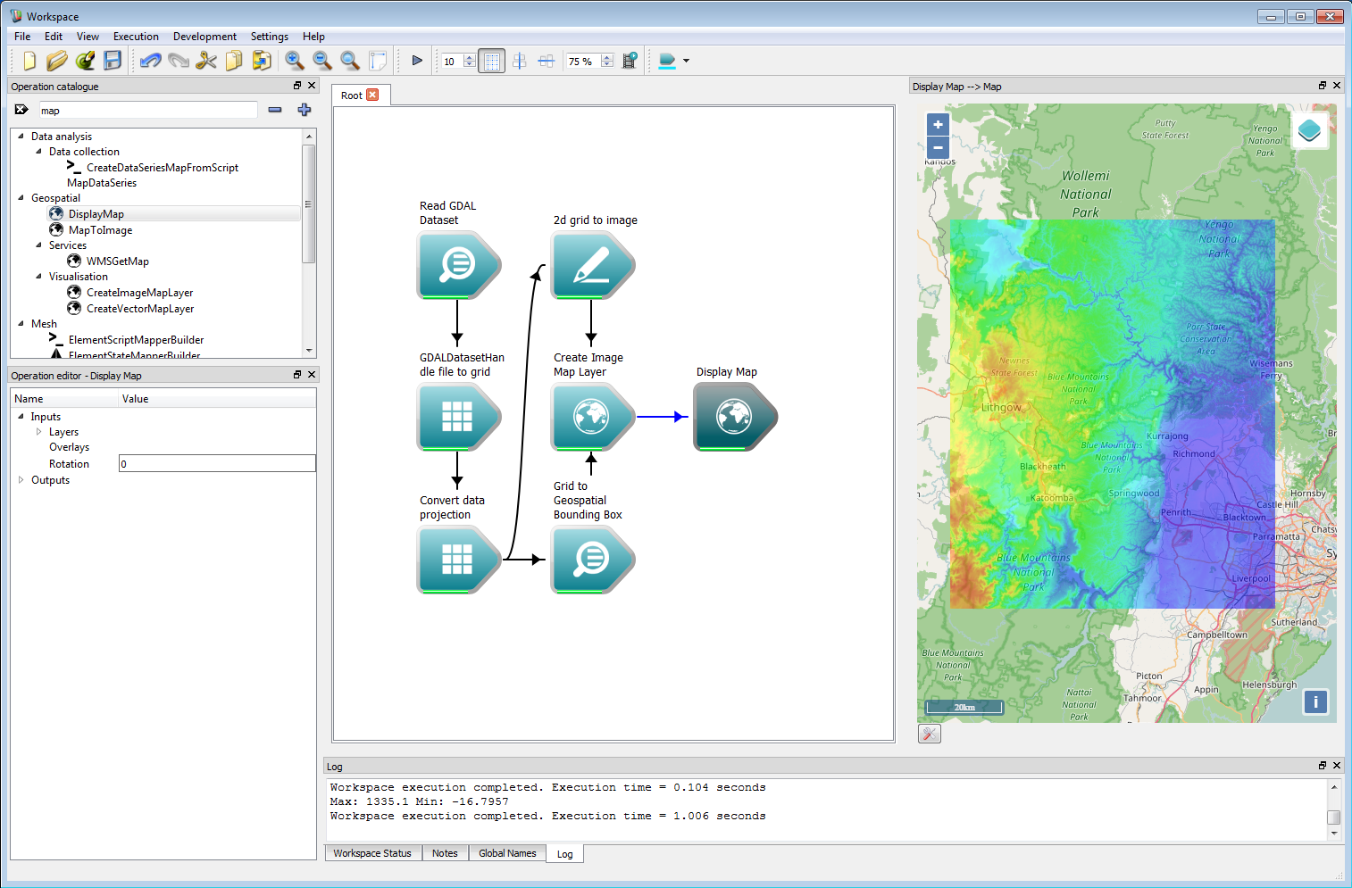Geospatial integration 4
The NetCDF data in this example can easily be used as a layer in a fire simulation. In the work-flow shown below, the elevation data is used to create a user data layer called 'elevation'. This is directly referenced in the rate-of-spread model, which is used here to give an unrealistic but illustrative fire perimeter. The starting location for the fire is given for simplicity in eastings and northings in MGA zone 56. The Arrival time output of the Bushfire solver operation is connected to a 2d grid to mesh operation, which converts the grid into a vector contour depending on the Height cut-off input (named 'height' for legacy reasons). The Height cut-off is set to zero in the operation, and the Create contour only box is checked. The resulting Meshmodel output is converted from MGA zone 56 to Spherical Mercator in the Create Vector Map Layer operation. The output from this operation is connected to the Layers input on the Display Map operation.

Geospatial integration 5

Note
If the input data has a time component Spark will automatically use a spatially and temporally interpolated value in the speed function calculation. This allows time-varying spatial grids from, for example, meteorological NetCDF files to be directly referenced in the speed function. The simulation start time can be set using the Simulation start time input of the bushfire configuration (as an ISO 8601 date stamp), all temporal sampling in the solver will be set relative to this.

Warning
If the start time does not specify a UTC time zone the local system time will be used. To ensure portability of workflows the UTC time zone should be specified.
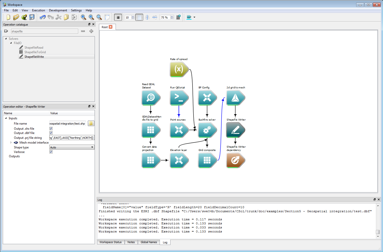
The vector output shown in the last example can be written directly to a ESRI shape-file using the ShapefileWrite operation. Optionally, a corresponding projection file can also be written with this operation from a text string.

Geospatial integration 6
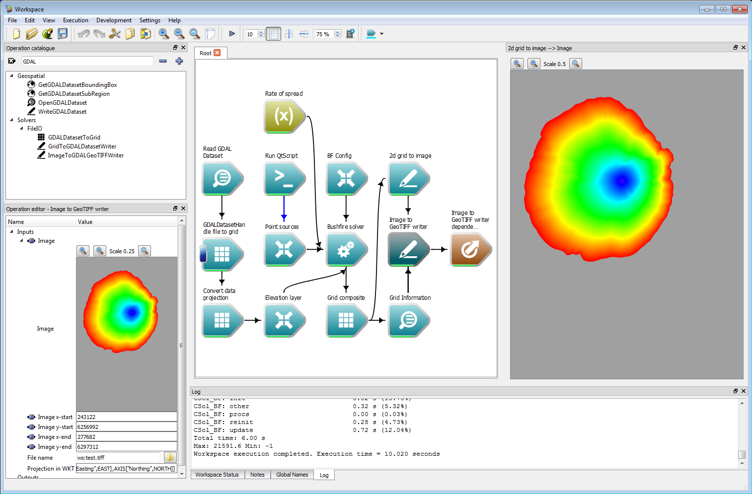
Another possible output format is a GeoTIFF file. Spark contains a specific Image to GeoTIFF writer which correctly handles transparent image regions. This requires a geospatial bounding box specified as the Image start and Image end inputs. This can be set using the origin and limit outputs of the Grid Information operation. The Image to GeoTIFF writer can also optionally store a projection specified as an OGC WKT (well-known text) string.

Geospatial integration 7
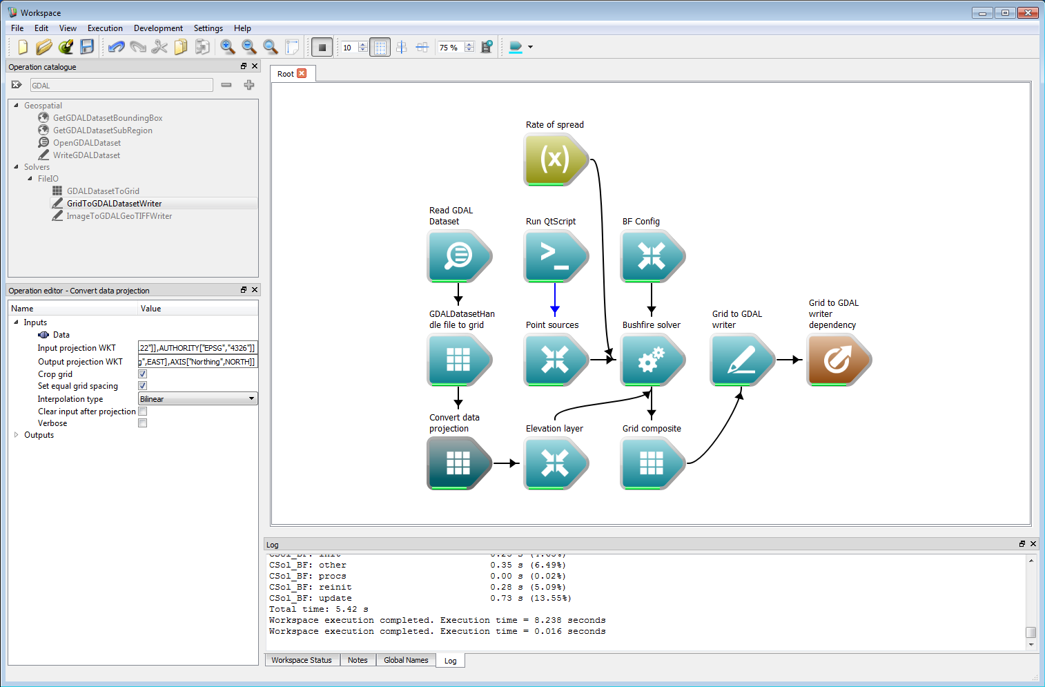
Raster layers can also be directly written using GDAL by the Grid to GDAL writer operation. This requires the GDAL output format, data format and an optional format and compression string. The format and compression strings are passed to GDAL as the FORMAT= and COMPRESS= parameters, respectively, in the creation options. Please refer to the GDAL documentation for valid arguments for these parameters. If these are blank, the default GDAL arguments are used. An optional projection can also be given as a OGC WKT (well-known text) string.

Geospatial integration 8
Vector and raster outputs can then be imported into QGIS, Google Earth or any other suitable GIS tool.

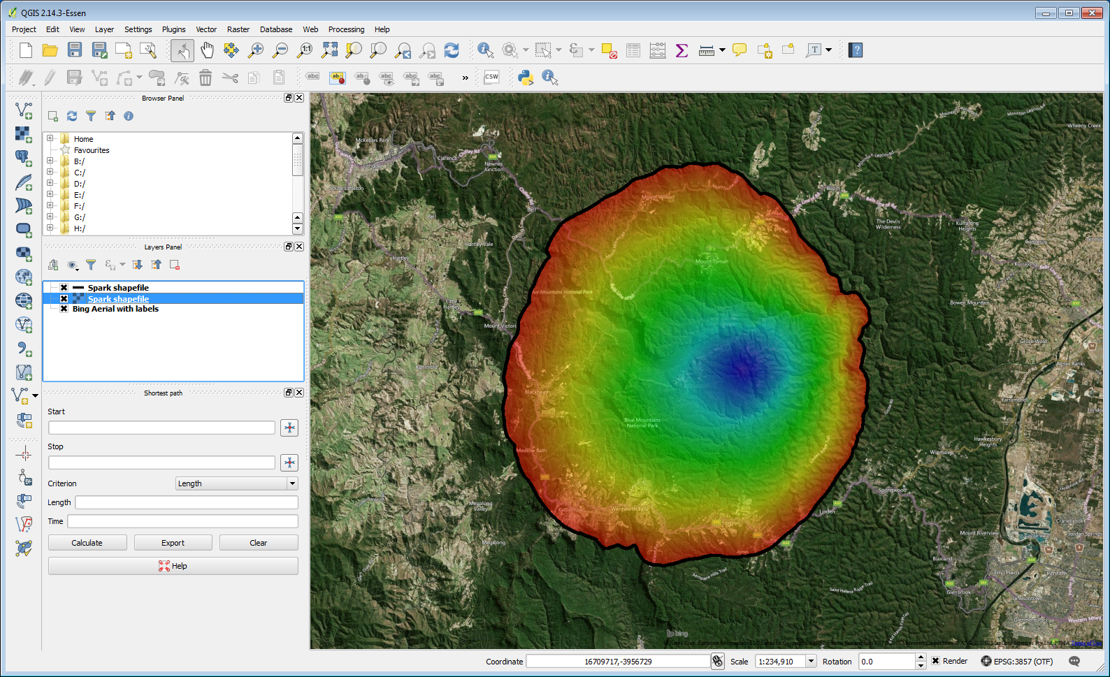Geospatial integration 9

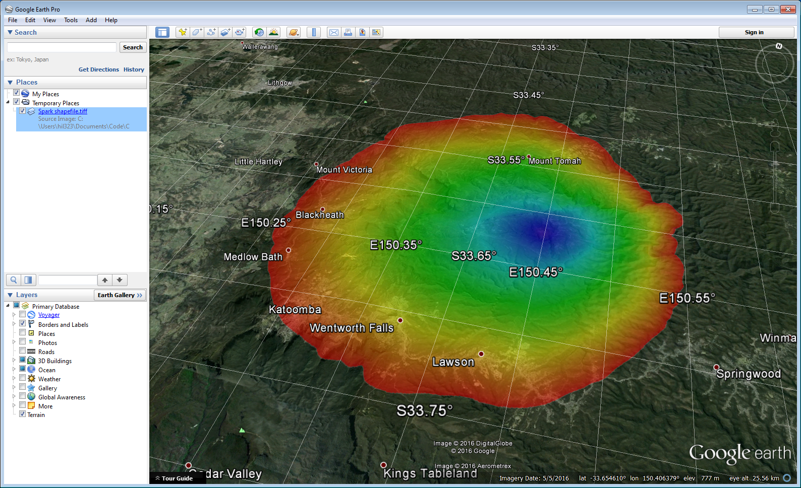Geospatial integration 10

Initialisation and post-processing models

Example files.

Spark supports additional user-programmable models for both initialisation of layers and post-processing for regions within the fire perimeter. The initialisation has already been covered in some examples, and can be used for a wide variety of purposes including local suppression, ecological modelling of fuel types and fuel accumulation. The post processing model can be used for combustion models such as flame height, smoke emission and heat flux. Internal variables which can be used in each of the programmable models are shown in the table below.

Variable	Type	Description	Used in*
easting	scalar	The cell easting value (m).	I
northing	scalar	The cell northing value (m).	I
speed	scalar	Required: sets the normal speed at the perimeter (m/s).	RP
wind	scalar	The dot product of the wind and front normal, limited by zero (m/s).	R
wind_vector	vector	The wind vector (m/s).	R
normal_vector	vector	The normal vector of the perimeter.	R
class	scalar	The cell classification value.	IRP
random	scalar	A random number from a uniform distribution between 0-1.	IRP
user0	scalar	Internal user-defined data layer, written to 'output grid' layer 0.	IRP
user1	scalar	Internal user-defined data layer, written to 'output grid' layer 1.	IRP
user2	scalar	Internal user-defined data layer, written to 'output grid' layer 2.	IRP
arrival	scalar	The ignition (arrival) time of the perimeter at the cell (s).	P
time	scalar	The current solver time (s).	RP
layername	scalar	The interpolated cell value of user-defined layer named layername.	IRP
dx(layername)	scalar	The x-spatial derivative of the user-defined layer named layername.	IR
dy(layername)	scalar	The y-spatial derivative of the user-defined layer named layername.	IR
grad(layername)	vector	The gradient of the user-defined layer named layername.	IR

I: Initialization programs, R: Rate-of spread programs, P: Post-processing programs

Warning: The post-processing model only operates within the fire perimeter.

Note: The restriction of three internal user defined layers will be lifted in future versions.

An example of using an initialisation model to build a fuel layer is shown in the following figure. A user-defined layer representing fuel age called burn_time is shown in the lower right panel, where black has a time since last burnt of zero and white is one (in arbitrary units). The grey areas indicate an intermediate time since last burnt. An empty layer called fuel_height is created and initialised using the fuel age data in the initialisation model. In this example, the fuel age is assumed to follow an inverse decay curve of 1-exp(-kt), where t is the fuel age. A special un-burnable (classification value zero) is used for the case of burn_time = 0. The perimeter speed function in this case is equal to the fuel_height squared. The resulting arrival time coloured from red (earliest) to blue (latest) is shown in the top right panel. The code for the initialisation model is:
if (burn_time == 0.0) {

class = 0;

}

fuel_height = 1-exp(-5*pow(burn_time, 2));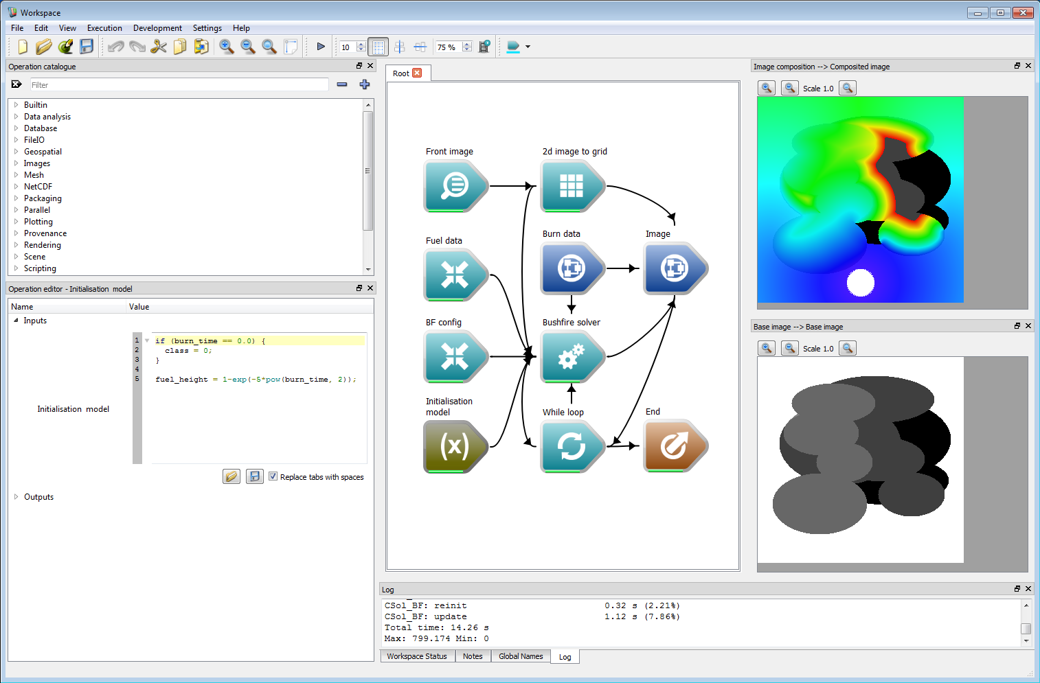

Fuel layer initialisation example
A second example of using an initialisation model based on location is shown in the following figure. In this case a perimeter expands from the origin at 0 m east and 0 m north. The initialisation model sets cells to be un-burnable within a circle of radius 100 m centred at 100 m east and 100 m north. The resulting arrival time coloured from red (earliest) to blue (latest) is shown in the right panel, where The perimeter has expanded around the un-burnable region. Initialisation models such as this can be used to programmatically alter fuel or classification states within the model without requiring additional fuel layers. The code for the initialisation model is:
if (hypot(easting-100, northing-100)<100.0) {

class = 0;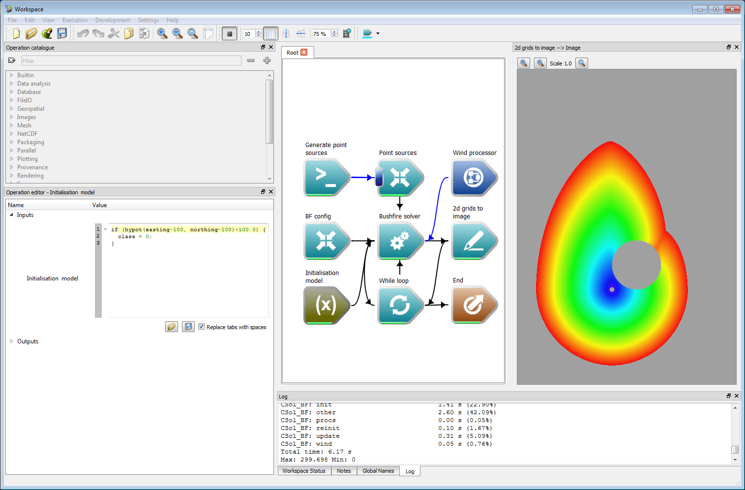

}

Location-based initialisation example
An example of using a post-processing model to calculate heat flux is shown in the following figure. In this basic model the flux is assumed to depend exponentially on fuel load in the cell, a heat of combustion and a mean burn time parameter. To calculate the flux the time since ignition is required. This is determined from the arrival variable, which is the cell ignition time, and the time variable, which is the current time. The difference between these is the length of time the cell has been ignited, which can be used in the heat flux expression. The panel on the right shows the resulting flux from three ignition points coloured from black (zero) to yellow (maximum). The post processing model could also be used to generate output layers for flame height or smoke emission. Like the speed function, the post-processing input accepts multiple models. Each of these models is run of the corresponding classification. The code for the post-processing model is:
REAL M = 10.0; // Fuel load (kg/m^2)

REAL H = 10.0E6; // Heat of combustion (J/kg)

REAL T = 10.0; // Mean burn time (s)

output0 = M*H*exp(-(time-arrival)/T)/T; // J/(s m^2)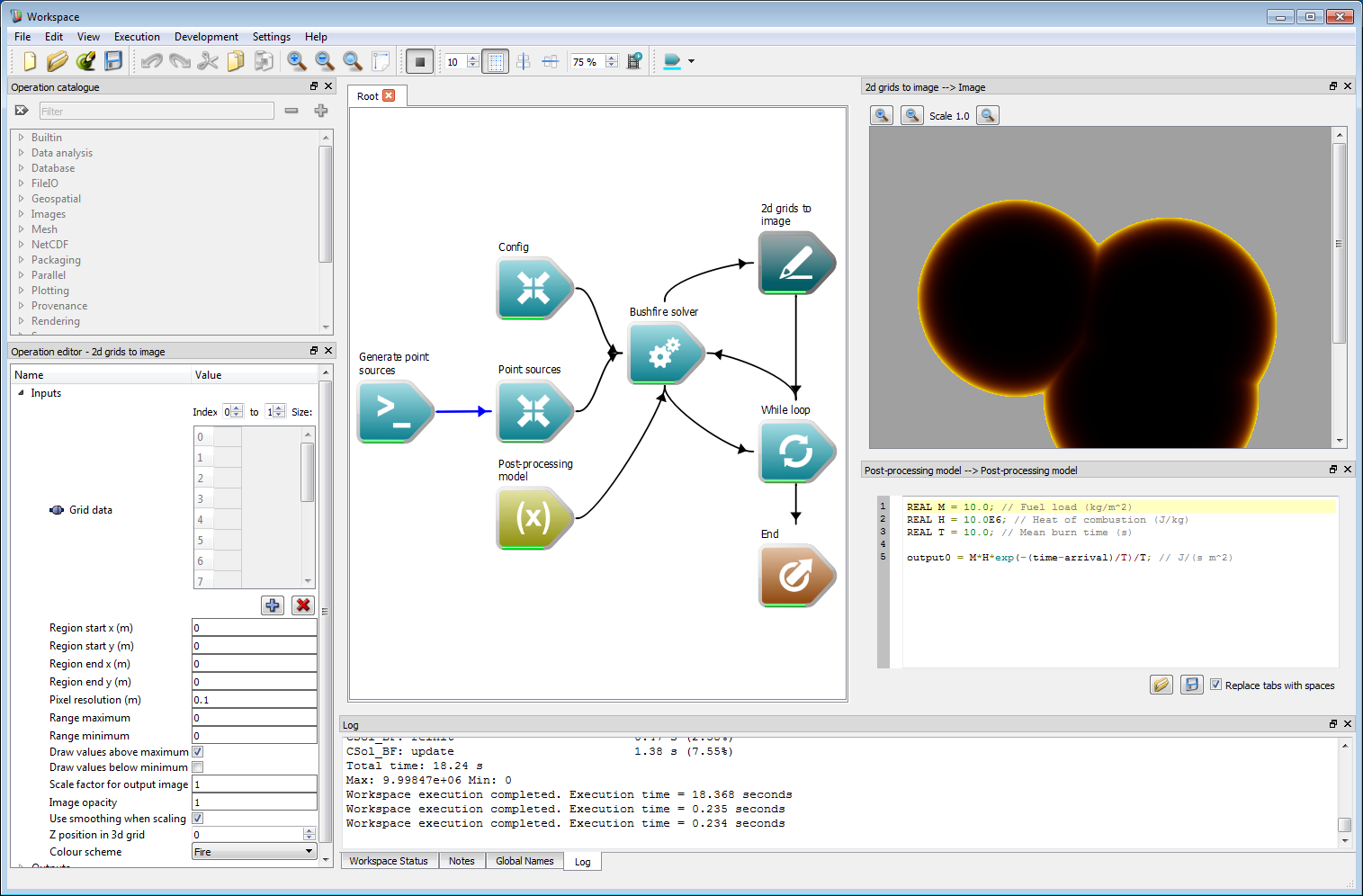

Post-processing model example

Summary

The examples shown here are only a fraction of the capability of the Spark framework. We hope that these basic examples have shown the flexibility of the system for a wide range of different applications.

[ Up: index ] [ Next: docswift ]

Contents

Introduction

Basic bushfire work-flow

Incorporating geospatial data

Interactive control

Ensemble analysis

Geospatial integration

Initialisation and post-processing models

Summary